Spin diffusion
The interaction of spin polarized currents with the magnetization can be described by a spin-accumulation model described in [Zhang2002] and [Garcia2007]. In this model the spin accumulation \(\vec{s}(\vec{x})\) exerts a torque on the magnetization by an additional term to the LLG
where \(J\) the coupling strength between itinerant and lattice magentic moments. The spin accumulation itself depends on the magnetization by the diffusion equation
where \(D_0\) is the diffusion constant, \(\tau_\text{sf}\) is the spin-flip relaxation time, and \(\mat{J}_\text{s}\) is the matrix valued spin current given by
Here \(\beta\) and \(\beta'\) are dimensionless polarization parameters and \(\mat{J}_\text{e}\) is the electrical current density. As shown in [Abert2014b] this method is able to reproduce the results of both the spin torque model by Slonczewski, see [Slonczewski1996], and the model by Zhang and Li, see [Zhang2004].
magnum.fe provides different methods for the solution of the spin diffusion model. The SpinDiffusion class integrates the dynamic spin diffusion equation. Combined with an Alouges type integrator it can be shown that the resulting scheme is unconditionally convergent, see [Abert2014a], [Abert2015].
The typical time scale of the motion of the spin accumulation is two orders of magnitude faster than that of the magnetic motion. Hence, if one is only interested in the magnetization dynamics it is reasonable to treat the spin accumulation in equilibrium by solving for the static case. This model is provided by the SpinAccumulationForCurrent class. It basically offers a method s() that can be registered as virtual attribute in order to provide the equilibrium spin accumulation for a given magnetization and current distribution.
Both models mentioned above require the prescription of an electric current density. However, the electric conductivity and thus also the current density is known to depend on the magnetization. A fully self-consistent model would therefore not only solve for the spin accumulation, but also for the electric current. The spin-diffusion model introduced above has its origin in a more general model, that was also introduced in [Zhang2002] where the electric current \(\vec{J}_\text{e}\) and the spin current \(\vec{J}_\text{s}\) are given by the coupled system
with \(\vec{E}\) being the electric field and \(C_0\) being connected to the electric conductivity \(\sigma\) by \(C_0 = \sigma/2\). Furthermore it is assumed that the electric field has a scalar potential \(u\) given by \(\vec{E} = - \nabla u\) and that there are no sources of electric current within the considered region \(\nabla \cdot \vec{J}_\text{e} = 0\). Plugging into the static equation for the spin accumulation \(\frac{\partial \vec{s}}{\partial t} = 0\) yields the system
which can be simultaneously solved for the potential \(u\) and the spin accumulation \(\vec{s}\). This is done by the SpinAccumulationForPotential class that provides methods for the computation of \(u\), \(\vec{s}\) and the electric current \(\vec{J}_\text{e}\). The details of this method are described in [Abert2016].
The SpinAccumulationWithSpinhall solver extends the SpinAccumulationForPotential solver by the spin Hall and invsere spin Hall effect. The spin current and electric current without spin Hall \(\vec{J}_\text{s}^0\) and \(\vec{J}_\text{e}^0\) are defined along the lines of the self-consistent model
According to [Dyakonov2007] the system including spin Hall effects is then given by
where \(\theta\) is the dimensionless spin Hall angle.
Any of these solvers provide methods to compute the spin accumulation for a given magnetization. In order to account for the influence of the spin accumulation onto the magnetization dynamics you have to include the SpinTorque term in the list of effective field contributions and make sure that the computed value for the spin accumulation is accessible via state.s.
An overview over the different spin diffusion classes is given in the following table:
| Class | \(\text{d}\vec{s}/\text{d}t = 0\) | self-consistent | (inverse) spin Hall |
|---|---|---|---|
SpinDiffusion |
no | no | no |
SpinAccumulationForCurrent |
yes | no | no |
SpinAccumulationForPotential |
yes | yes | no |
SpinAccumulationWithSpinhall |
yes | yes | yes |
Legacy material parameters
Until version 1.1.x, magnum.fe implemented all spin diffusion models with a different set of material parameters. Namely instead of the coupling strength \(J\) and the spin-flip relaxation time \(\tau_\text{sf}\) the former formulation includes the coupling constant \(c\) and the diffusion lengths \(\lambda_\text{sf}\) and \(\lambda_\text{J}\). With these parameters the extended LLG reads
and the dynamics of the spin accumulation \(\vec{s}\) are described by
where \(\lambda_\text{sf}\) is the characteristic length for spin-flip relaxation and \(\lambda_\text{J}\) depends on the electron’s mean free path. Note, that three legacy parameters (\(c\), \(\lambda_\text{sf}\), and \(\lambda_\text{J}\)) are substituted by two parameters (\(J\) and \(\tau_\text{sf}\)) which means, that the legacy set of parameters is overdefined. The old parameters are still supported, but magnum.fe will print a legacy warning and it is recommended to switch to the new set of parameters. The following relations between old and new parameters hold
Cell and facet regions
All spin diffusion related classes require the definition of certain cell and facet regions, see Fig. 17. As usual, regions containing magnetic material have to be included in the magnetic region. Moreover, all conducting materials have to be included in the conducting region. Note that conducting magnetic regions have to be included in this region, too.
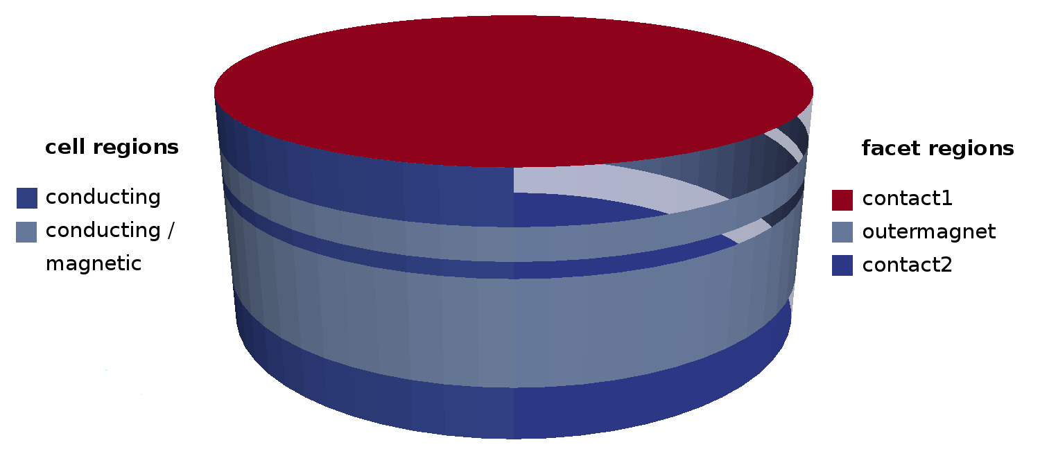
Fig. 17 Regions required by the different spin diffusion classes. The facet regions contact1 and contact2 are only required by the SpinAccumulationForPotential class in order to apply a potential to the stack.
Besides the cell regions all spin diffusion classes require the definition of a outermagnet facet region. This region should contain all interfaces between air and magnetic material. In the case of a magnetic multilayer that is surrounded contacted with nonmagnetic electrodes, this region includes the side facets of the magnetic layers (not the metal-magnetic interfaces).
Note that the definition of the outermagnet region only influences the simulation if the region is passed by an electric current. The defintion can be omitted if this is not the case.
See the figure for the proper definition of both cell and facet regions for a magnetic/nonmagnetic multilayer stack.
SpinDiffusion
-
class
magnumfe.SpinDiffusion(magnetic_region='magnetic', conducting_region='conducting', outermagnet_region='outermagnet')¶ Solver for the spin-diffusion equation according to [Abert2014a]. The spin diffusion \(\vec{s}\) is computed from the current magnetization \(\vec{m}\) by
\[\begin{split}\int_{\Omega} \;\text{d}_{t} \boldsymbol{s}^{k+1} \cdot \boldsymbol{\zeta} \;\text{d}\boldsymbol{x} \;+\; a(\boldsymbol{s}^{k+1}, \boldsymbol{\zeta}) =\\ \frac{\beta \mu_\text{B}}{e} \int_{\omega} \left[ \boldsymbol{m}^{k+1} \otimes \boldsymbol{j}^{k+1} \right] : \boldsymbol{\nabla} \boldsymbol{\zeta} \;\text{d}\boldsymbol{x} - \frac{\beta \mu_\text{B}}{e} \int_{\partial \Omega \cap \partial \omega} (\boldsymbol{j}^{k+1} \cdot \boldsymbol{n}) (\boldsymbol{m}^{k+1} \cdot \boldsymbol{\zeta}) \;\text{d}\boldsymbol{x}\end{split}\]where \(\text{d}_t \vec{s}^{k+1} = (\vec{s}^{k+1} - \vec{s}^k)\) and the bilinear form \(a(\zeta_1, \zeta_2)\) is defined as
\[\begin{split}a(\boldsymbol{\zeta_1}, \boldsymbol{\zeta_2}) = \frac{1}{\tau_\text{sf}} \int_{\Omega} \boldsymbol{\zeta}_1 \cdot \boldsymbol{\zeta}_2 \;\text{d}\boldsymbol{x} + 2 D_0 \int_{\Omega} \boldsymbol{\nabla} \boldsymbol{\zeta}_1 : \boldsymbol{\nabla} \boldsymbol{\zeta}_2 \;\text{d}\boldsymbol{x} \\ - 2 D_0 \beta \beta' \int_{\omega} \left[ \boldsymbol{m}^{k+1} \otimes \left((\boldsymbol{\nabla} \boldsymbol{\zeta}_1)^T \boldsymbol{m}^{k+1} \right) \right] : \boldsymbol{\nabla} \boldsymbol{\zeta}_2 \;\text{d}\boldsymbol{x} + \frac{J}{\hbar} \int_{\omega} \left( \boldsymbol{\zeta}_1 \times \boldsymbol{m}^{k+1} \right) \cdot \boldsymbol{\zeta}_2 \;\text{d}\boldsymbol{x}.\end{split}\]The region \(\Omega\) corresponds to the “conducting” cell domain and the region \(\omega\) corresponds to the “magnetic” cell domain. The boundary \(\partial \Omega \cap \partial \omega\) has to be defined explicitly as facet domain named “outermagnet”.
The characteric time scale of the spin-diffusion dynamics is orders of magnitude smaller than that of the magnetization dynamics. However, the integration scheme is able to handle very large time steps. Hence the time step can be taken from the integration of the LLG if only the magnetization dynamics are of interest, see [Abert2014b].
Add the
SpinCurrentto the LLG terms in order to get a bidirectional coupling of spin diffusion and magnetization.- Example
# initialize integrators
llg      = LLGAlougesProject([ExchangeField()])
spindiff = SpinDiffusion()

# perform integration step of size 1ps
state.step([llg, spindiff], 1e-12)
- Arguments
- magnetic_region (
str) - magnetic region, defaults to ‘magnetic’
- conducting_region (
str) - conducting region, defaults to ‘conducting’
- outermagnet_region (
str) - facet region that marks magnet/air interfaces, defaults to ‘outermagnet’
- magnetic_region (
SpinAccumulationForCurrent
-
class
magnumfe.SpinAccumulationForCurrent(magnetic_region='magnetic', conducting_region='conducting', outermagnet_region='outermagnet', solver='gmres', prec='default')¶ This class represents the coupling of the magnetization with a spin polarized current. The spin accumulation is treated in equilibrium. The current has to prescribed in the state.
- Arguments
- magnetic_region (
str) - Name of the magnetic region
- conducting_region (
str) - Name of the conducting region
- outermagnet_region (
str) - Name of the outer-magnet facet region
- solver (
str) - Solver for linear system (“bicgstab”, “gmres”,...), defaults to “gmres”
- prec (
str) - Preconditioner for linear system (“ilu”, “amg”, ...), default to “ilu”
- magnetic_region (
- Example
# Initialize state with magnetization
state = State(...)
state.m = Constant((1.0, 0.0, 0.0))

# Set constant current
state.j = Constant((1e12, 0.0, 0.0))

# Create solver and hook into state
spin_acc = SpinAccumulationForCurrent()
state.s = spin_acc.s()
- Required fields
- m
- Magnetization
- j
- Electric Current
- Required material parameters
- D0
- Diffusion constant
- beta
- Polarization parameter
- beta_prime
- Polarization parameter
- tau_sf
- Spin-flip relaxation time
- J
- exchange strength between itinerant and localized spins
SpinAccumulationForPotential
-
class
magnumfe.SpinAccumulationForPotential(magnetic_region='magnetic', conducting_region='conducting', outermagnet_region='outermagnet', solver='bicgstab', prec='default')¶ Computes the equilibrium spin accumulation s, the electric potential u and the electric current j for a given magnetization configuration and mixed boundary conditions for the potential.
- Example
# Initialize state with magnetization
state = State(...)
state.m = Constant((1.0, 0.0, 0.0))

# set a constant current inflow on contact1 facet-region
state.j_boundary = {'contact1': Constant(1e12)}

# set a constant potential on contact2 facet-region
state.u_boundary = {'contact2': Constant(0.0)}

# Create solver and hook into state
spin_acc = SpinAccumulationForPotential()
state.s = spin_acc.s()
state.j = spin_acc.j()
- Arguments
- magnetic_region (
str) - Name of the magnetic region, defaults to “magnetic”
- conducting_region (
str) - Name of the conducting region, defaults to “conducting”
- outermagnet_region (
str) - Name of the outer-magnet facet region
- solver (
str) - Solver for linear system (“bicgstab”, “gmres”,...), defaults to “bicgstab”
- prec (
str) - Preconditioner for linear system (“ilu”, “amg”, ...), default to “ilu”
- magnetic_region (
- Required fields
- m
- Magnetization
- u_boundary
- Potential boundary conditions
- j_boundary
- Current boundary conditions
- Required material parameters
- D0
- Diffusion constant
- C0
- Connected to the electrical conductivity \(\sigma\) by \(C_0 = \sigma/2\)
- beta
- Polarization parameter
- beta_prime
- Polarization parameter
- tau_sf
- Spin-flip relaxation time
- J
- exchange strength between itinerant and localized spins
-
j(state=None)¶ Returns the electric current for a given state.
- Arguments
- state (
State) - The state. If state is not provided a lambda for use as virtual state attribute is returned.
- state (
- Returns
dolfin.Functionorlambda- Electric current or lambda
-
js(state=None)¶ Returns the spin current for a given state.
- Arguments
- state (
State) - The state. If state is not provided a lambda for use as virtual state attribute is returned.
- state (
- Returns
dolfin.Functionorlambda- Spin current or lambda
SpinAccumulationWithSpinhall
-
class
magnumfe.SpinAccumulationWithSpinhall(magnetic_region='magnetic', conducting_region='conducting', outermagnet_region='outermagnet', solver='bicgstab', prec='default')¶ Computes the equilibrium spin accumulation s, the electric potential u and the electric current j for a given magnetization configuration and mixed boundary conditions for the potential. Takes into account spin Hall and inverse spin Hall effect due to the spin Hall angle \(\theta\).
- Example
# Initialize state with magnetization
state = State(...)
state.m = Constant((1.0, 0.0, 0.0))

# set a constant current inflow on contact1 facet-region
state.j_boundary = {'contact1': Constant(1e12)}

# set a constant potential on contact2 facet-region
state.u_boundary = {'contact2': Constant(0.0)}

# Create solver and hook into state
spin_acc = SpinAccumulationForPotential()
state.s = spin_acc.s()
state.j = spin_acc.j()
- Arguments
- magnetic_region (
str) - Name of the magnetic region, defaults to “magnetic”
- conducting_region (
str) - Name of the conducting region, defaults to “conducting”
- outermagnet_region (
str) - Name of the outer-magnet facet region
- solver (
str) - Solver for linear system (“bicgstab”, “gmres”,...), defaults to “bicgstab”
- prec (
str) - Preconditioner for linear system (“ilu”, “amg”, ...), default to “ilu”
- magnetic_region (
- Required fields
- m
- Magnetization
- u_boundary
- Potential boundary conditions
- j_boundary
- Current boundary conditions
- Required material parameters
- D0
- Diffusion constant
- C0
- Connected to the electrical conductivity \(\sigma\) by \(C_0 = \sigma/2\)
- beta
- Polarization parameter
- beta_prime
- Polarization parameter
- tau_sf
- Spin-flip relaxation time
- J
- exchange strength between itinerant and localized spins
- theta
- spin Hall angle
-
j(state=None)¶ Returns the electric current for a given state.
- Arguments
- state (
State) - The state. If state is not provided a lambda for use as virtual state attribute is returned.
- state (
- Returns
dolfin.Functionorlambda- Electric current or lambda
| [Zhang2002] | (1, 2) Zhang, S., Levy, P. M., & Fert, A. (2002). Mechanisms of spin-polarized current-driven magnetization switching. Physical review letters, 88(23), 236601. |
| [Garcia2007] | García-Cervera, C. J., & Wang, X. P. (2007). Spin-polarized currents in ferromagnetic multilayers. Journal of Computational Physics, 224(2), 699-711. |
| [Abert2014b] | (1, 2) Abert, C., Ruggeri M., Bruckner F., Vogler C., Hrkac G., Praetorius D., & Suess D. (2014). Self-consistent micromagnetic simulations including spin diffusion effects. In preparation |
| [Slonczewski1996] | Slonczewski, J. C. (1996). Current-driven excitation of magnetic multilayers. Journal of Magnetism and Magnetic Materials, 159(1), L1-L7. |
| [Zhang2004] | Zhang, S., & Li, Z. (2004). Roles of nonequilibrium conduction electrons on the magnetization dynamics of ferromagnets. Physical Review Letters, 93(12), 127204. |
| [Abert2014a] | (1, 2)
|
| [Abert2015] | Abert, C., Ruggeri, M., Bruckner, F., Vogler, C., Hrkac, G., Praetorius, D., & Suess, D. (2015). A three-dimensional spin-diffusion model for micromagnetics. Scientific reports, 5. |
| [Abert2016] | Abert, C. to be published |
| [Dyakonov2007] | Dyakonov, M. I. (2007). Magnetoresistance due to edge spin accumulation. Physical review letters, 99(12), 126601. |