A Simple Spin-Torque Oscillator¶

In this section the simulation of a simple spin torque oscillator is shown in order to demonstrate the handling of multiple domains in magnum.fe.

Load Mesh and Name Regions¶

We use the mesh, that we created in Creating a multilayer structure with Gmsh. Like in any magnum.fe simulation script we have to include the magnum.fe library. In the next line the mesh is loaded from the file stack.xml.

from magnumfe import *

mesh = Mesh("stack.xml")

The mesh file contains domain information through numbered IDs as pointed out in the preceding section. For convenience, magnum.fe offers the possibility to assign names to these regions. Some region names are important for the default behaviour of magnum.fe. For instance, the LLG is by default always solved in the region named ‘magnetic’, the spin accumulation is by default solved on the ‘conducting’ region. Moreover, arbitrary names might by assigned to regions in order to simplify material assignment or postprocessing operations such as computing averages. The name assignment is done on the creation of the state object. Cell domains and facet domains are treated individually.

state = State(mesh,
  cell_domains = {
    'electrode_bottom': 1,
    'fixed_layer':      2,
    'spacer':           3,
    'free_layer':       4,
    'electrode_top':    5,
    'magnetic':         (2,4),
    'conducting':       (1,2,3,4,5)
  },
  facet_domains = {
    'contact_bottom':   1,
    'contact_top':      2
  },
  scale = 1e-9
)

A single domain ID may be assigned to multiple named domains. In the next step material constants for the different regions (cell domains) are defined.

Define Material Constants¶

Depending on the models and field contributions to be solved, the definition of different constants is required. Material constants can either be scalar, such as the saturation magnetization ms, or vector valued, such as the easy axis of the uniaxial anisotropy field. Material constants are discretized by piecewise constant functions. That means, that material parameters are constant within each simulation cell.

# Define material constants in magnetic region
state.material['magnetic'] = Material(
  alpha      = 0.1,
  Aex        = 2.8e-11,
  D0         = 1e-3,
  C0         = 1.2e6,
  beta       = 0.9,
  beta_prime = 0.8,
  tau_sf     = 5e-14,
  J          = 4.0e-20
)

# Define specific constants for free layer
state.material['free_layer'] = Material(
  ms         = 1.00 / Constants.mu0,
  K_uni      = 0.0,
  K_uni_axis = (0, 0, 1)
)

# Define specific constants for fixed layer
state.material['fixed_layer'] = Material(
  ms         = 1.24 / Constants.mu0,
  K_uni      = 1e6,
  K_uni_axis = (0, 0, 1)
)

# Define material constants for nonmagnetic region
state.material['!magnetic'] = Material(
  D0         = 5e-3,
  C0         = 6e6,
  tau_sf     = 1e-14,
)

Note that the material parameters are applied in the order of appearance. Parameters, set in certain regions can be overridden by subsequent calls of the material setter. The nonmagnetic region in this example is referred to by application of the inversion operator ‘!’, e.g. ‘!magnetic`. Important parameter constants for the magnetic region are the damping alpha, the exchange constant Aex, the saturation magnetization ms and the anisotropy constant K_uni and axis K_uni_axis. All constants are given in SI units (e.g. saturation magnetization in A/m, Aex in J/m).

Initialize and Relax Magnetization¶

Next the initial magnetization configuration is defined. Again, domain names can be used to conveniently set the magnetization in the individual regions.

state.m = state.interpolate({
            'free_layer':  Constant((1.0, 0.0, 0.0)),
            'fixed_layer': Constant((0.0, 0.0, 1.0))
          })

Instead of Constant objects we could also have used spatially varying Expression objects as in the standard problem #4 example. Now that we have defined an initial magnetization configuration, the magnetization should be relaxed into an energetic minimum. We start by defining effective-field contributios that should be considered for energy minimization.

exchange_field = ExchangeField()
demag_field    = DemagField()
aniso_field    = UniaxialAnisotropyField()
external_field = ExternalField(Constant((0.0, 0.0, 0.6 / Constants.mu0)))

Next, an LLG integrator is initialized with the defined fields, the damping of the system is set to \(\alpha = 1\) for a fast relaxation, and the LLG is integrated a couple of steps.

llg = LLGCvode([exchange_field, demag_field, aniso_field, external_field])
state.material['magnetic'].alpha = 1.0
for i in range(100): state.step(llg, 1e-11)

Due to the high damping, the system is considered to be in equilibrium after 1ns.

Couple Spin-Diffusion Model to LLG¶

Now, we want to add a DC current to the system to obtain an oscillation in the free layer. The most advanced model in magnum.fe for description of the interaction of electric current and magnetization is the self-consistent spin accumulation model supplied by the class SpinAccumulationForPotential. It provides solvers for the spin accumulation that takes boundary conditions like current inflow or electric potential as an input and computes not only the spin accumulation, but also the electric potential and current. In order to make the spin accumulation available to the SpinTorque LLG term it is registered in the state object as a virtual attribute.

spin_acc = SpinAccumulationForPotential()
state.s  = spin_acc.s()
state.j  = spin_acc.j()
state.u  = spin_acc.u()

Moreover, the suppliers for the electric current j and the potential u are registered. As mentioned above, the SpinAccumulationForPotential class requires boundary conditions for the computation of the different fields. These boundary conditions are also registered in the state as virtual attributes.

state.j_boundary = {'contact_top':    Constant(4e11)}
state.u_boundary = {'contact_bottom': Constant(0.0)}

At the top contact, a constant current outflow of \(4 \cdot 10^{11}\) A/m is defined. The bottom contact is assigned zero electric potential. Note that due to the DC current these virtual attributes are simply constants. Virtual attributes in general may depend on the simulation state in an arbitrary fashion. An AC current outflow could be easily implemented by state.j_boundary = lambda state: Constant(A*sin(2*pi*freq*state.t)) with A being the amplitude and freq being the frequency.

Now everything is set up to compute the spin accumulation, but there is still a lack of an LLG contribution that couples the spin accumulation to the magnetization dynamics. This job is done by the the SpinTorque class that implements a torque term that expects the spin accumulation to be supplied by state.s.

spin_torque    = SpinTorque()

Adding this term to an LLG integrator enables the solution of the coupled LLG and spin diffusion equation. In order to simulate the oscillation, the damping is set back to \(\alpha = 0.1\) and the time of the state is reset to 0.

llg = LLGCvode([exchange_field, demag_field, aniso_field, external_field, spin_torque])
state.material['magnetic'].alpha = 0.1
state.t = 0.0

Now log files for the scalar data and the fields magnetization \(\vec{m}\), spin accumulation \(\vec{s}\), and current \(\vec{j}\) are created.

# prepare log files
logger  = ScalarLogger("log.dat", ('t', 'm[free_layer]', 'u[facet:contact_top]'))
mlogger = FieldLogger("data/m.pvd", 'm[magnetic]', every = 10)
slogger = FieldLogger("data/s.pvd", 's', every = 10)
jlogger = FieldLogger("data/j.pvd", 'j', every = 10)

Beside the fields and the averaged magnetization, we are interested in the conductivity of the stack depending on the magnetization configuration. Since the self-consistent model solves for the potential in the whole sample, the conductivity can be easily obtained by computing the potential difference of the top contact to the bottom contact. The potential at the bottom contact is set to 0 in the simulation script. The potential at the top contact can be easily logged by adding a column u[facet:contact_top] to the logger. The complete integration code including logging then reads

while state.t < 4e-9:
  logger  << state
  mlogger << state
  slogger << state
  jlogger << state

  state.step(llg, 1e-11)

Results¶

The applied current is expected to move the magnetization in the free layer out of its equilibrium configuration which leads to oscillation. The system will then reach a dynamic equilibrium where the energy dissipation is exactly compensated by the constant current, see Figure. The potential difference \(u\) is expected to be relatively small in the beginning of the simulation, where the magnetization in the free layer is almost parallel to the fixed layer and then increases and saturates when reaching the stable oscillation mode, see Fig. 14.

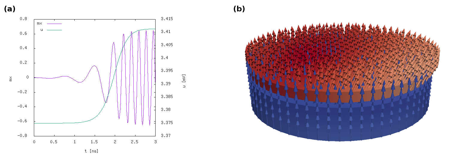
Fig. 14 Results for the spin torque oscillator. (a) Time development of the average magnetization and potential difference of top to bottom contact. (b) snapshot of the magnetization during oscillation.