Field Terms¶

Effective field terms and extensions to the LLG are represented by the LLGTerm class. magnum.fe comes with a number of predefined LLGTerm classes that cover a variety of use cases. As shown in the previous section, a list of FieldTerm objects is usually passed to an LLG integrator object in order to integrate the LLG under the influence of different effects. Moreover each LLGTerm object has methods to compute the corresponding effective field and energy for a given State object.

# initialize state with uniform magnetization configuration
state = State(mesh, m = Constant((1.0, 0.0, 0.0)))

# initialize demagnetization field object
demag = DemagField()

# compute field and save to file
File("h.pvd") << demag.h(state)

# compute energy and print on screen
print demag.E(state)

Both, the field method h and the energy method E can also be used as virtual attribues.

state.h_demag = demag.h()
state.E_demag = demag.E()

Computation of the field can be restricted to a certain region. Usually, the default region for is the ‘magnetic’ region. This default can be overriden in the initializer in order to solve for the field in another region.

exchange = ExchangeField(region = 'ferromagnetic')

Some of the predefined LLGTerm classes describe nonlocal fields, e.g. the DemagField and the OerstedField class. These classes additionally distinguish between a source region and target region.

# compute field generate by the free layer in the free layer
DemagField(region = 'free_layer')

# compute field generate by the fixed layer in the free layer
DemagField(source_region = 'fixed_layer', target_region = 'free_layer')

Some LLGTerm classes require certain material parameters to be defined, e.g. the exchagne field requires the exchange constant Aex and the saturation magnetization ms. Please refer to the following reference documentation for detailed information on the individual llg terms.

`LLGTerm`¶

class magnumfe.LLGTerm(preconditionable=False, region='magnetic', lump=True, m_order=None, has_energy=True, weight='ms', form_cache_keys=set(['material']), result_cache_keys=set(['m']))¶

Superclass of all effective field contributions. Subclasses should at least implement the form method.

Arguments

region (str): The region where the field is evaluated, defaults to ‘magnetic’.
lump (bool): Flag, if True the projection is computed with a lumped mass matrix (faster)
m_order (int): Order of the magnetization in the energy used for automated energy calculation. By default this value is guessed from the form, however this might fail if auxiliary expressions are used.
has_energy (bool): Should be set to False by an inheriting class that does not support energy computation (e.g. spin torque). In that case the E method throws an exception.
weight (function): A function that returns a multiplicator for the field projection method. Defaults to material.ms which should be the correct choice for eny local energy contribution, e.g. exchange field.
form_cache_keys (set): Cache keys for the matrix/vector assembly from the form for the field computation
result_cache_keys(set): Cache keys for the result of the field computation

E(state=None)¶

Return the energy connected with the field contribution, if implemented in the subclass. This method can either be called directly or registered as virtual attribute.

Arguments

state (State): the state

Returns

float: the energy

form_lhs(state, dt_v)¶

Returns the left-hand-side contribution of the effective field for Alouges-type integration schemes.

Arguments

state (State): The simulation state.
dt_v (dolfin.TrialFunction): The trial function multiplied with the timestep and theta.

Returns

dolfin.Form: the form contribution for the LHS

form_rhs(state)¶

Returns the right-hand-side contribution of the effective field for Alouges-type integration schemes.

Arguments

state (State): The simulation state.

Returns

dolfin.Form: the form contribution for the RHS

h(state=None, x=None)¶

Returns the effective-field contribution for a given state. This method can either be called directly or registered as virtual attribute.

Uses a projection method to retrieve the field from the RHS-form given by the form_rhs method. It should be overriden for better performance.

Arguments

state (State): the simulation state
x (dolfin.Vector): the vector to store the result or None

Returns

dolfin.Function: the effective-field contribution

prec_form(state)¶: Returns the m-dependent contribution to the preconditioner. Defaults to :code`form_rhs`.

prec_region()¶: Returns additional regions that have to be taken into account for preconditioning.

prec_setup(state, m)¶: Preprocesses RHS of preconditioning system.

`AFCoupling`¶

class magnumfe.AFCoupling(A, direction, interface='af', region='magnetic')¶

This class represents the coupling of a ferromagnetic interface to an antiferromagnet. The antiferromagnet is usually not included in the ‘magnetic’ region. It might even be omitted completely if it is not required for other computations such as the electric current distribution.

The coupling is initialized by defining an interface, a coupling direction (preferred direction of the magnetization in the magnetic region) and a coupling constant.

Fig. 15 Interface definition for antiferromagnetic coupling.

Arguments

A (float): Coupling constant in \(J/m^2\)
direction (dolfin.GenericFunction): Direction of the coupling, e.g. Constant((1, 0, 0))
interface (str): Name of the facet domain where the coupling is applied
region (str): The region where the field is evaluated, defaults to ‘magnetic’.

Required fields

m: Magnetization

`CompositeTerm`¶

class magnumfe.CompositeTerm(*terms)¶

This class combines multiple LLGTerm objects to a single object for the convenient calculation of the overall field and energy.

Note

The resulting object is not suitable for use in LLGCvode since preconditioning capabilities are lost.

Example

exchange = ExchangeField()
demag    = DemagField()
total    = CompositeTerm(exchange, demag)

total.h(state)
total.E(state)

Arguments

*terms (LLGTerm): The LLGTerms to be combined to a single term.

`CubicAnisotropyField`¶

class magnumfe.CubicAnisotropyField(region='magnetic', lump=True)¶

This class represents a second order uniaxial anisotropy field.

\[\begin{split}\vec{H} = - \frac{2 K_1}{\mu_0 M_\text{s}} \mat{A}(\alpha, \beta, \gamma) \begin{pmatrix} m_1 m_2^2 + m_1 m_3^2\\ m_2 m_3^2 + m_2 m_1^2\\ m_3 m_1^2 + m_3 m_2^2 \end{pmatrix} - \frac{2 K_2}{\mu_0 M_\text{s}} \mat{A}(\alpha, \beta, \gamma) \begin{pmatrix} m_1 m_2^2 m_3^2 \\ m_1^2 m_2 m_3^2 \\ m_1^2 m_2^2 m_3 \end{pmatrix}\end{split}\]

where \(\mat{A}(\alpha, \beta, \gamma)\) is a rotation matrix with \(\alpha\), \(\beta\) and \(\gamma\) being the Euler angles:

\[\begin{split}\mat{A}(\alpha, \beta, \gamma) = \begin{pmatrix} \cos \alpha \cos \gamma - \sin \alpha \cos \beta \sin \gamma & -\cos \alpha \sin \gamma - \sin \alpha \cos \beta \cos \gamma & \sin \alpha \sin \beta \\ \sin \alpha \cos \gamma + \cos \alpha \cos \beta \sin \gamma & -\sin \alpha \sin \gamma + \cos \alpha \cos \beta \cos \gamma & -\cos \alpha \sin \beta \\ \sin \beta \sin \gamma & \sin \beta \cos \gamma & \cos \beta \end{pmatrix}\end{split}\]

The Euler angles are optional. If not provided, the are assumed to be zero and the easy axes coincide with the coordinate axes.

Arguments

region (str): The region where the field is evaluated, defaults to ‘magnetic’.
lump (bool): Flag, if True the projection is computed with a lumped mass matrix (faster)

Required fields

m: magnetization

Required material parameters

ms: saturation magnetization
K1_cubic: anisotropy constant
K2_cubic: anisotropy constant
K_cubic_alpha (optional): Euler angle alpha
K_cubic_beta (optional): Euler angle beta
K_cubic_gamma (optional): Euler angle gamma

`DemagField`¶

class magnumfe.DemagField(method='Fredkin Koehler', order=1, solver='LU', region=None, lump=True, source_region=None, target_region=None, compute_region=None, **kwargs)¶

Solves for the magnetic demagnetization field. The connected open boundary problem can either be solved with a hybrid FEM/BEM method (Fredkin Koehler) or a shell transformation method (Shell Transform). For most cases the FEM/BEM coupling is preferrable. For details, see Open Boundary Problems.

Arguments

lump (bool): Flag, if True the projection is computed with a lumped mass matrix (faster)
method (str): Method for the solution of the open-boundary problem. Possible Values are “Fredkin Koehler”/”FK” and “Shell Transform”/”ST”
order (int): The order of CG function used for the potential calculation. Currently only affects ST method.
solver (str): Solver type for FEM systems (either “LU” or “CG”). Currently only affects FK method.
region (str): Region where sources are considered and the field is evaluated. Defaults to ‘magnetic’ if non of region, source_region and target_region are given.
source_region (str): If given, only sources in this region are considered for field computation. Requires definition of target_region.
target_region (str): If given, field is only evaluated in this region. Requires definition of source_region.
compute_region (str): If given, FEM/BEM problem is solved in this region. Must contain both source_region and target_region.
aca_eps (float): Accuracy of ACA algorithm. FK method only.
bem_quad_degree_near (float): BEM quadrature degree for triangles with small distance, defaults to 4
bem_quad_degree_medium (float): BEM quadrature degree for triangles with medium distance, defaults to 3
bem_quad_degree_far (float): BEM quadrature degree for triangles with large distance, defaults to 2

Required fields

m: Magnetization

Required material parameters

ms: saturation magnetization in A/m

u(state)¶

Calculate the demagnetization-field potential u for a given simulation state

Arguments

state (State): The simulation state

`ExchangeField`¶

class magnumfe.ExchangeField(region='magnetic', lump=True)¶

This class represents the micromagnetic exchange field.

Arguments

region (str): The region where the field is evaluated, defaults to ‘magnetic’.
lump (bool): Flag, if True the projection is computed with a lumped mass matrix (faster)

Required fields

m: Magnetization

Required material parameters

ms: saturation magnetization in A/m
Aex: exchange constant in J/m

`ExternalField`¶

class magnumfe.ExternalField(h=Coefficient(FunctionSpace(None, VectorElement(FiniteElement('Real', None, 0), dim=3)), 0), region='magnetic')¶

This class represents an external field. The field value can either be a constant or a lambda depending on the time.

Example

# Define a constant field of 1T in x direction
external = ExternalField(Constant((1.0/Contants.mu0, 0.0, 0.0)))

# Define a field linearly varying in x direction
external = ExternalField(Expression(('x[0]', '0.0', '0.0')))

# Define an oscillating field
external = ExternalField(lambda t: Constant((A*sin(2*pi*freq*t), 0.0, 0.0)))

Arguments

h (dolfin.cpp.GenericFunction/lambda): The external field (GenericFunction or lambda)
region (str): The region where the field is evaluated, defaults to ‘magnetic’.

set(h)¶

Reset the field to a new value.

Arguments

h (dolfin.GenericFunction/lambda): the field

`InterfaceDMIField`¶

class magnumfe.InterfaceDMIField(region='magnetic', lump=True)¶

This class represents the interface Dzyaloshinskii-Moriya interaction corresponding to the energy

\[E = D [ m_\text{n} \vec{\nabla} \cdot \vec{m} - (\vec{m} \cdot \vec{\nabla}) m_\text{n} ]\]

with the coupling constant \(D\) and the projected magnetization \(m_\text{n}\) defined by

\[m_\text{n} = \vec{m} \cdot \vec{n}\]

where \(\vec{n}\) is a normalized direction vector (usually the interface normal).

Arguments

region (str): The region where the field is evaluated, defaults to ‘magnetic’.
lump (bool): Flag, if True the projection is computed with a lumped mass matrix (faster)

Required fields

m: Magnetization

Required material parameters

D_inter: DMI coupling constant
D_inter_axis: DMI axis (usually the interface normal)

`InterlayerExchange`¶

class magnumfe.InterlayerExchange(A, layer_region='interlayer_region', interface1='interface1', interface2='interface2', region='magnetic')¶

This class represents a Heisenberg-type coupling of two neighboring interfaces and can be used to model e.g. synthetic antiferromagnets.

The volume between these interfaces has to be meshed and marked as nonmagnetic. While the interfaces are not required to have the same number of nodes, they should be more or less in parallel and have the same size. Furthermore it is recommended to avoid interal mesh nodes within the coupling region since this requires an additional solver step for the evaluation of the effective field. The coupling constant is provided in J/m^2 and a positive constant means ferromagnetic coupling (negative constant means antiferromagnetic coupling).

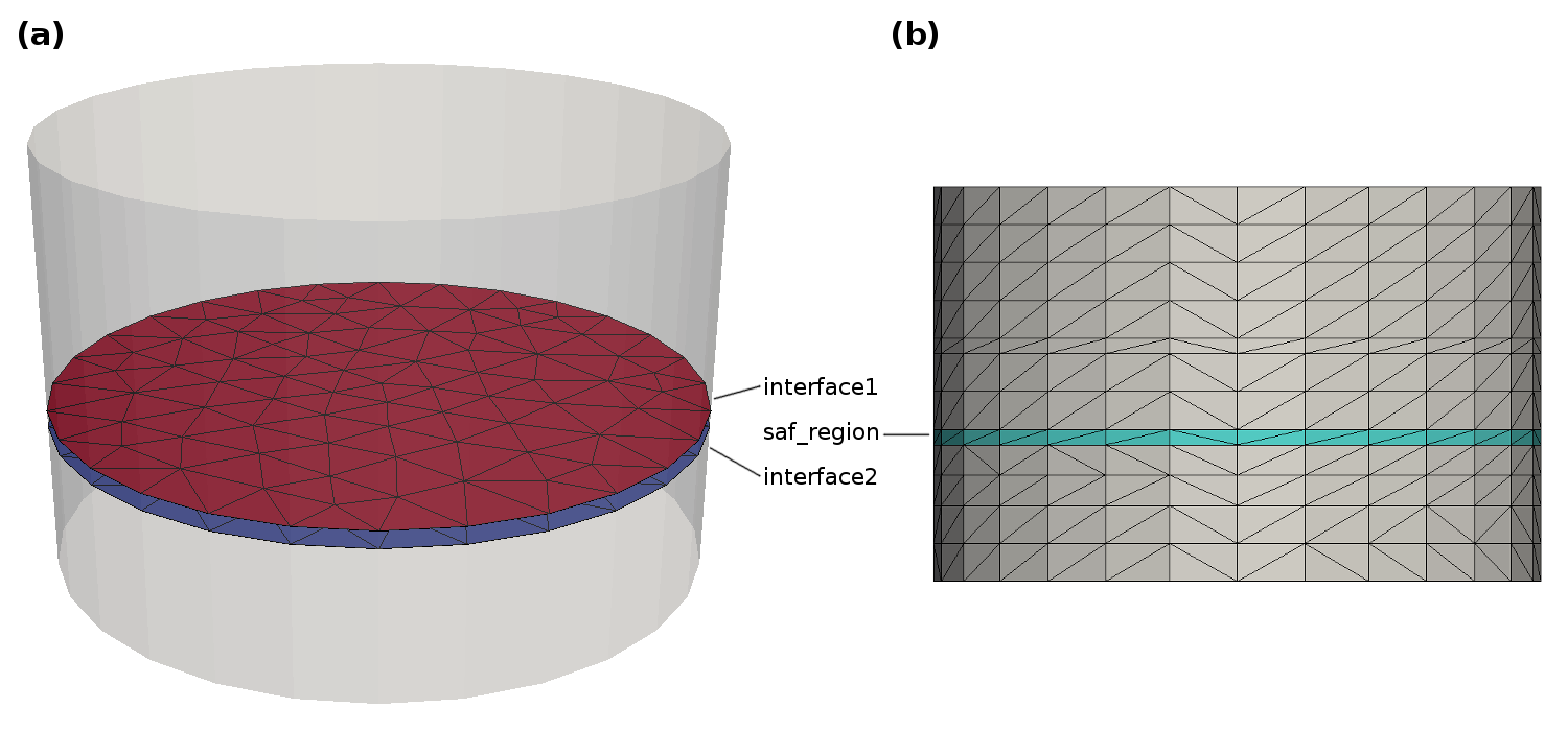
Fig. 16 Interface and region definition for a SAF layer. (a) interfaces (b) region.

Arguments

A (float): Coupling constant in J/m^2 (positive constant means ferromagnetic coupling)
saf_region (str): Name of the cell domain of the SAF layer
interface1 (str): Name of the facet domain of SAF layer interface 1
interface2 (str): Name of the facet domain of SAF layer interface 2
region (str): The region where the field is evaluated, defaults to ‘magnetic’.

Required fields

m: Magnetization

`OerstedField`¶

class magnumfe.OerstedField(method='Fredkin Koehler', order=1, solver='LU', region=None, source_region=None, target_region=None, compute_region=None, **kwargs)¶

Solves for the current indeced Oersted field. The connected open boundary problem can either be solved with a hybrid FEM/BEM method (Fredkin Koehler) or a shell transformation method (Shell Transform). For most cases the FEM/BEM coupling is preferrable. For details, see Open Boundary Problems.

Arguments

method (str): Method for the solution of the open-boundary problem. Possible Values are “Fredkin Koehler”/”FK” and “Shell Transform”/”ST”
order (int): The order of CG function used for the potential calculation.
solver (str): Solver type for FEM systems (either “LU” or “CG”). Currently only affects FK method.
region (str): Region where sources are considered and the field is evaluated. Defaults to ‘conducting’ if non of region, source_region and target_region are given.
source_region (str): If given, only sources in this region are considered for field computation. Requires definition of target_region.
target_region (str): If given, field is only evaluated in this region. Requires definition of source_region.
compute_region (str): If given, FEM/BEM problem is solved in this region. Must contain both source_region and target_region.
aca_eps (float): Accuracy of ACA algorithm. FK method only.
bem_quad_degree_near (float): BEM quadrature degree for triangles with small distance, defaults to 4
bem_quad_degree_medium (float): BEM quadrature degree for triangles with medium distance, defaults to 3
bem_quad_degree_far (float): BEM quadrature degree for triangles with large distance, defaults to 2

Required fields

j: Electric Current

`SAFLayer`¶

class magnumfe.SAFLayer(A, saf_region='saf', interface1='saf1', interface2='saf2', region='magnetic')¶

This class represents an antiferromagnetic coupling of two neighboring interfaces.

This class is deprecated. Use InterlayerExchange instead (note that InterlayerExchange uses a different sign for the coupling constant A.

Arguments

A (float): Coupling constant in J/m^2 (positive constant means antiferromagnetic coupling)
saf_region (str): Name of the cell domain of the SAF layer
interface1 (str): Name of the facet domain of SAF layer interface 1
interface2 (str): Name of the facet domain of SAF layer interface 2
region (str): The region where the field is evaluated, defaults to ‘magnetic’.

Required fields

m: Magnetization

`SpinTorque`¶

class magnumfe.SpinTorque(region='magnetic')¶

This class represents the coupling of the magnetization with a spin polarized current. It requires the spin accumulation s to be set in the state. The spin accumulation s has to be prescribed in the state, either by direct integration with SpinDiffusion or by equilibrium treatment with SpinAccumulationForCurrent or SpinAccumulationForPotential.

Arguments

region (str): The region where the LLG is solved, defaults to ‘magnetic’

Required fields

s: Spin accumulation

Required material parameters

J: exchange strength between itinerant and localized spins in J
ms: saturation magnetization in A/m

`SpinTorqueSlonczewski`¶

class magnumfe.SpinTorqueSlonczewski(layer_region='interlayer_region', interface1='interface1', interface2='interface2', interface=None, region='magnetic', method1=None, method2=None, method=None, M=None, **kwargs)¶

Computes the spin torque between two interfaces according to the model of Slonczewski. The interacting layers have to be connected by a nonmagnetic region as in the SAFLayer class. There are two predefined couplings which can be defined per interface. both couplings provide an effective field contribution of the form

\[\vec{h} = \eta(\theta) \frac{j_\text{e} \hbar}{2 e \mu_0 M_\text{s} t} \vec{m} \times \vec{M}\]

where \(j_\text{e}\) is the current directed towards the target interface, \(M\) is the magnetization in the source interface, and \(t\) is the local thickness of the simulation cell. The angular dependency \(\eta\) in the predefined models “default” and “general” is defined as follows:

default

\[\eta(\theta) = \frac{P \Gamma}{(\Gamma + 1) + (\Gamma - 1) \cos(\theta)}\]

additional Arguments (float)

P (\(P\)) for symmetric coupling or P1,P2 for asymmetric coupling
Gamma (\(\Gamma\)) for symmetric coupling or Gamma1,Gamma2 for asymmetric coupling

general

\[\eta(\theta) = \frac{q^+}{A + B \cos(\theta)} + \frac{q^-}{A - B \cos(\theta)}\]

additional Arguments (float)

qm (\(q^-\)) for symmetric coupling or qm1,qm2 for asymmetric coupling
qp (\(q^+\)) for symmetric coupling or qp1,qp2 for asymmetric coupling
A (\(A\)) for symmetric coupling or A1,A2 for asymmetric coupling
B (\(B\)) for symmetric coupling or B1,B2 for asymmetric coupling

The class can also be used to compute the torque on a single interface for a given polarization \(\vec{M}\). In this case there is no need for a layer region or a second interface.

Example

# Default model, symmetric spin torque
spintorque = SpinTorqueSlonczewski(
               layer_region = "spacer",
               interface1 = "i1",
               interface2 = "i2",
               P = 0.8, Gamma = 0.8)

# Default model, asymmetric spin torque
spintorque = SpinTorqueSlonczewski(
               layer_region = "spacer",
               interface1 = "i1",
               interface2 = "i2",
               P1 = 0.8, Gamma1 = 0.8,
               P2 = 0.7, Gamma2 = 0.7)

# General model applied only to interface 2
spintorque = SpinTorqueSlonczewski(
               layer_region = "spacer",
               interface1 = "i1",
               interface2 = "i2",
               method2 = "general",
               qm = 1, qp = 1, A = 0.5, B = 0.5)

# Simple model with predefined polarization M defined on single interface
# No need to set interface1, interface2 or layer_region
spintorque = SpinTorqueSlonczewski(
               interface = "i1",
               M = Constant((1., 0., 0.)),
               P = 0.8, Gamma = 0.8)

Arguments

layer_region (str): Region separating the involved interfaces
interface1 (str): First interface of spin torque junction
interface2 (str): Second interface of spin torque junction
interface (str): Interface for static torque (provided by M)
region (str): The region where the field is evaluated, defaults to ‘magnetic’
method (str | function): Specific spin-torque model. Applies to both interfaces. Possible values are “default” or “general” for predefined methods, see above, or functions implementing a custom method.
method1 (str | function): Spin-torque model for interface 1
method2 (str | function): Spin-torque model for interface 2

Required fields

m: magnetization
j: electric current

`SpinTorqueZhangLi`¶

class magnumfe.SpinTorqueZhangLi(region='magnetic')¶

Implements the the spin torque model of Zhang and LI [Zhang2004]. This model extends the LLG as follows

\[\partial_t \vec{m} = - \gamma ( \vec{m} \times \vec{H}_\text{eff} ) + \alpha ( \vec{m} \times \partial_t \vec{m} ) - b \vec{m} \times [\vec{m} \times (\vec{J} \cdot \nabla) \vec{m}] - b \xi \vec{m} \times (\vec{J} \cdot \nabla) \vec{m}\]

in order to describe the interaction of an electric current with the magnetization.

Arguments

region (str): The region where the field is evaluated, defaults to ‘magnetic’

Required fields

m: magnetization
j: electric current

Required material parameters

xi: degree of nonadiabacity
b: coupling constant

`UniaxialAnisotropyField`¶

class magnumfe.UniaxialAnisotropyField(region='magnetic')¶

This class represents a second order uniaxial anisotropy field.

\[\vec{H} = \frac{2 K_\text{uni}}{\mu_0 M_\text{s}} \vec{K}_\text{axis} (\vec{K}_\text{axis} \cdot \vec{m})\]

where \(\vec{K}_\text{axis}\) is the anisotropy axis.

Arguments

region (str): The region where the field is evaluated, defaults to ‘magnetic’.

Required fields

m: magnetization

Required material parameters

ms: saturation magnetization
K_uni: anisotropy constant
K_uni_axis: anisotropy axis, e.g. (1, 0, 0)

[Zhang2004]

Zhang, S., & Li, Z. (2004). Roles of nonequilibrium conduction electrons on the magnetization dynamics of ferromagnets. Physical Review Letters, 93(12), 127204.