Solvers

The following classes provide different solvers for specific tasks.

Electric Potential

class magnumfe.ElectricPotential(magnetic_region='magnetic', conducting_region='conducting', outermagnet_region='outermagnet', solver='cg', prec='default')

Computes the electric potential and current according to Ohm’s law. Boundray conditions can be given either as potential (Dirichlet) or current outflow (Neumann).

Example

# Initialize state with magnetization
state = State(...)

# set a constant current inflow on contact1 facet-region
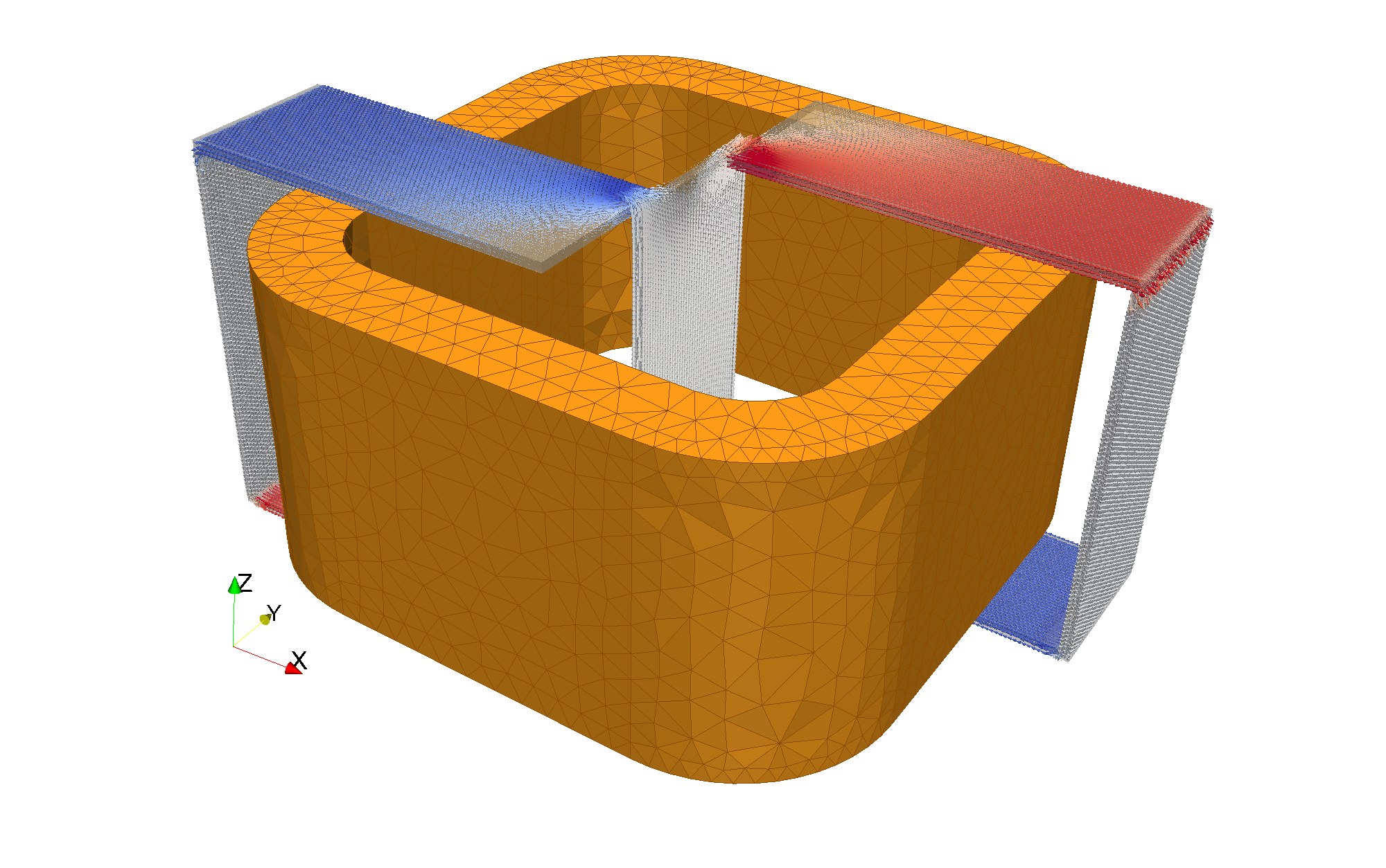
state.j_boundary = {'contact1': Constant(1e12)}

# set a constant potential on contact2 facet-region
state.u_boundary = {'contact2': Constant(0.0)}

# Create solver and hook into state via virtual attributes
potential = ElectricPotential()
state.u = potential.u()
state.j = potential.j()

Arguments

conducting_region (str)

Name of the conducting region, defaults to “conducting”

solver (str)

Solver for linear system (“cg”, “gmres”,...), defaults to “bicgstab”

prec (str)

Preconditioner for linear system (“ilu”, “amg”, ...), default to “ilu”

Required fields

u_boundary

Potential boundary conditions

j_boundary

Current boundary conditions

Required material parameters

sigma

Electric conductivity

C0

Alternative to conductivity, see SpinAccumulationForPotential (\(C_0 = \sigma/2\))

j(state=None)

Returns the electric current for a given state.

Arguments

state (State)

The state. If state is not provided a lambda for use as virtual state attribute is returned.

Returns

dolfin.Function or lambda

Electric current or lambda

Maxwell Solvers

Different methods are available for the solution of the magnetostatic Maxwell equations:

\[\begin{split}\text{rot} \vec{H} &= \vec{j} \quad \text{in} \; \Omega_m \\ \text{div} \vec{B} &= 0 \quad \text{in} \; \Omega_m\end{split}\]

The open-boundary problem is handled by the direct Johnson-Nedelec FEM-BEM coupling method, which avoids the discretization of the other domain. The following jump conditions need to be considered at the surface of the magnetic material:

\[\begin{split}\vec{n} \times \left[\![ \vec{H} \right]\!] &= 0 \\ \vec{n} \cdot \left[\![ \vec{B} \right]\!] &= 0\end{split}\]

The magnetic flux density \(\vec{B}\) and the magnetic field \(\vec{H}\) are connected via a (nonlinear) material law. For the numerical solutioin with a Newton-like method, the material law is linearized around the actual bias point:

\[\vec{B} = \vec{B}(\vec{H}) \approx \vec{B}_\text{r} + \chi \, \vec{H}\]

At the moment only \(H\)-based methods are implemented. The source of these methods is an external field \(H_\text{ext}\) (sometimes called impressed current vector potential). Any FieldTerm class can be used to create the source field for a Maxwell problem. If for example a known current density should act as sources of the magnetic field the OerstedField class can be used to calculate \(H_\text{ext}\).

MaxwellReduced

Since the external field \(H_\text{ext}\) contains all rotational contibutions to the total field which are created by some current distribution, the remaining induced field \(H_\text{d}\) is irrotational and can therefor be described by a gradient field:

\[\vec{H} = \vec{H_{ext}} - \nabla u\]

The reduced scalar potential \(u\) can be defined globally and always exists. Unfortunately cancelation effects can occur if magnetic materials with high susceptibility are considered. In this case the induced field and the external field nearly cancel each other, which may lead to large numerical errors. Nevertheless the reduced scalar potential is often useful due to its simplicity.

\[\begin{split}\vec{\nabla} \cdot \left(\vec{\mu} \, \vec{\nabla} u \right) &= \vec{\nabla} \cdot \left( \mu \, \vec{H_{ext}} + \vec{B}_\text{r}\right) \quad \text{in} \; \Omega \\ \Delta u &= 0 \quad \text{in} \; \mathbb{R}^3 \setminus \Omega \\ [\![ u ]\!] &= 0 \quad \text{on} \; \partial \Omega \\ [\![\nabla u \cdot \vec{\mu} \cdot \vec{n} ]\!] &= \left( \vec{H_{ext}} \cdot [\![ \mu ]\!] + \vec{B}_\text{r} \right) \cdot \vec{n} \quad \text{on} \; \partial \Omega\end{split}\]

Using the direct Johnson-Nedelec FEM-BEM coupling method leads to the following discretized system of equations:

\[\begin{split}\begin{pmatrix} M^{11}_{ij} & M^{12}_{in} \\ M^{21}_{mj} & M^{22}_{mn} \end{pmatrix} \begin{pmatrix} u_j \\ \phi_n \end{pmatrix} = \begin{pmatrix} RHS^1_i \\ \vec{0} \end{pmatrix}\end{split}\]

\[\begin{split}M^{11}_{ij} &= \int\limits_{\Omega} \mu^+ \, \vec{\nabla} \Lambda_i \cdot \vec{\nabla} \Lambda_j \, d\Omega \\ M^{12}_{in} &= -\int\limits_{\Gamma} \Lambda_i \, \mathbb{1}_n \, d\Gamma \\ M^{21}_{mj} &= \frac{1}{2} \Lambda_j(\vec{x}_m) - \frac{1}{4 \pi} \int\limits_{\Gamma} \Lambda_j(\vec{y}) \frac{\vec{x}_m - \vec{y}}{\vert \vec{x}_m - \vec{y}\vert^3} \, \vec{n} \, d\Gamma_y \\ M^{22}_{mn} &= \frac{1}{4 \pi} \int\limits_{\Gamma} \frac{\mathbb{1}_n(\vec{y})}{\vert \vec{x} - \vec{y}\vert} \, d\Gamma_y \\ RHS^1_{i} &= -\int\limits_{\Gamma} \mu_0 \, \vec{H}_\text{ext} \cdot \vec{n} \, \Lambda_i \, d\Gamma + \int\limits_{\Omega} \left( \vec{H}_\text{ext} \cdot \mu + \vec{B}_\text{r} \right) \cdot \nabla \Lambda_i \, d\Omega\end{split}\]

From the mathematical point of view using piecewise linear and continuous basis functions \(\Lambda_i\) for the potential and piecewise constant basis functions \(\mathbb{1}_n\) for the normal derivative seems to be the natural choice for a lowest order discritization. Nevertheless the Johnson-Nedelec coupling should be stable for arbitrary combinations of function spaces.

class magnumfe.MaxwellReduced(lump=True, region='maxwell', tol=1e-16, maxiter=20)

This class solves the magnetostatic Maxwell equations using a reduced scalar potential formulation as introduced in [Bruckner2012].

Example

mesh = UnitCubeMesh(10,10,10)
state = State(mesh, scale = 1e-9)
state.maxwell_material = MaxwellMaterial.Linear(chi=1e3)
state.Hext = ExternalField(Constant((0.0, 0.0, 1.0))).h(state)

solver = MaxwellReduced()
Hd = solver.Hd(state)
Htot = solver.Htot(state)
M = solver.M(state)
B = solver.B(state)

Note

The external field is assumed to be in state.Hext.

Note

This class requires the PETSc Backend to be enabled.

Arguments

lump (bool)

Flag, if set to True external field terms are computed with mass lumping

prec_solver (string)

Solver for preconditioning system, either ‘LU’ or ‘GMRES’, defaults to ‘LU’

region (string)

The region where the Maxwell equations are solved, defaults to ‘maxwell’

tol (float)

Threshold for the tolerance within the Newton iteration

maxiter (int)

Maximum number of Newton iterations

u(state=None)

Calculate \(\vec{m}(H_{ext})\).

Arguments

state (State)

The external field configuration.

MaxwellTotal

An alternative scalar potential formulation, which does not suffer from numerical cancelation errors, is the total scalar potential. In contrast to the reduced scalar potential, the total scalar potential directly describes the total field:

\[\vec{H} = - \nabla u\]

Since this formulation is only allowed in regions without current density, it is necessary to devide the global problem into inner and other region. While the total scalar potential can only be defined within the inner region, a reduced scalar potential is used to describe the outer region (where some currents are needed to create the source field \(H_\text{ext}\). Additionally the total scalar potential is only well defined if the inner region is singly-connected (artificial cuts can be used to create a singly-connected domain). Furthermore since the potential description changes from inner to outer region the formulatioin of the jump conditions at the boundary of the magnetic domain, requiers the knowledge of a potential of the external field \(u_\text{ext}\). Putting everything together the following equations can be derived for the total scalar potential:

\[\begin{split}\vec{\nabla} \cdot \left(\vec{\mu} \, \vec{\nabla} u \right) &= \vec{\nabla} \cdot \vec{B}_\text{r} \quad \text{in} \; \Omega \\ \Delta u &= 0 \quad \text{in} \; \mathbb{R}^3 \setminus \Omega \\ [\![ u ]\!] &= u_\text{ext} \quad \text{on} \; \partial \Omega \\ [\![\nabla u \cdot \vec{\mu} \cdot \vec{n} ]\!] &= \left( -\mu_0 \, \vec{H_{ext}} + \vec{B}_\text{r} \right) \cdot \vec{n} \quad \text{on} \; \partial \Omega\end{split}\]

Using the direct Johnson-Nedelec FEM-BEM coupling method leads to the following discretized system of equations:

\[\begin{split}\begin{pmatrix} M^{11}_{ij} & M^{12}_{in} \\ M^{21}_{mj} & M^{22}_{mn} \end{pmatrix} \begin{pmatrix} u_j \\ \phi_n \end{pmatrix} = \begin{pmatrix} RHS^1_i \\ RHS^2_m \end{pmatrix}\end{split}\]

\[\begin{split}M^{11}_{ij} &= \int\limits_{\Omega} \mu^+ \, \vec{\nabla} \Lambda_i \cdot \vec{\nabla} \Lambda_j \, d\Omega \\ M^{12}_{in} &= -\int\limits_{\Gamma} \Lambda_i \, \mathbb{1}_n \, d\Gamma \\ M^{21}_{mj} &= \frac{1}{2} \Lambda_j(\vec{x}_m) - \frac{1}{4 \pi} \int\limits_{\Gamma} \Lambda_j(\vec{y}) \frac{\vec{x}_m - \vec{y}}{\vert \vec{x}_m - \vec{y}\vert^3} \, \vec{n} \, d\Gamma_y \\ M^{22}_{mn} &= \frac{1}{4 \pi} \int\limits_{\Gamma} \frac{\mathbb{1}_n(\vec{y})}{\vert \vec{x}_m - \vec{y}\vert} \, d\Gamma_y \\ RHS^1_{i} &= -\int\limits_{\Gamma} \mu_0 \, \vec{H}_\text{ext} \cdot \vec{n} \, \Lambda_i \, d\Gamma + \int\limits_{\Omega} \vec{B}_\text{r} \cdot \nabla \Lambda_i \, d\Omega\\ RHS^2_{i} &= M^{21}_{mj} \, u_j^\text{ext}\end{split}\]

class magnumfe.MaxwellTotal(lump=True, region='maxwell')

This class solves the magnetostatic Maxwell equations using a total scalar potential formulation as introduced in [Bruckner2012].

Example

mesh = UnitCubeMesh(10,10,10)
state = State(mesh, scale = 1e-9)
state.maxwell_material = MaxwellMaterial.Linear(chi=1e3)
state.Hext = ExternalField(Constant((0.0, 0.0, 1.0))).h(state)

solver = MaxwellTotal()
Hd = solver.Hd(state)
Htot = solver.Htot(state)
M = solver.M(state)
B = solver.B(state)

Note

The external field is assumed to be in state.Hext.

Note

This class requires the PETSc Backend to be enabled.

Arguments

lump (bool)

Flag, if set to True external field terms are computed with mass lumping

prec_solver (string)

Solver for preconditioning system, either ‘LU’ or ‘GMRES’, defaults to ‘LU’

region (string)

The region where the Maxwell equations are solved, defaults to ‘maxwell’

u(state=None)

Calculate \(\vec{m}(H_{ext})\).

Arguments

state (State)

The external field configuration.

StringSolver

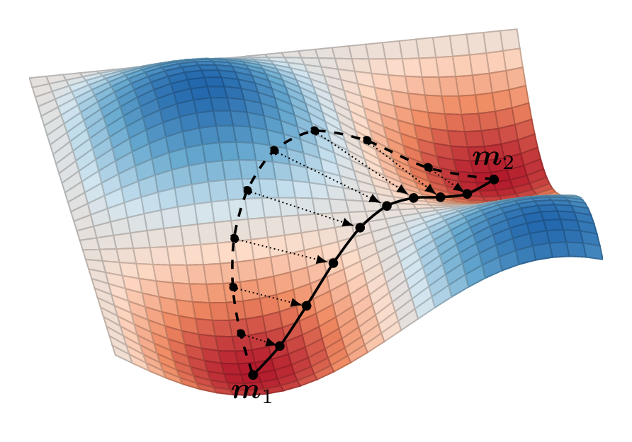
magnum.fe implements the string method as introduced in [E2007] for the computation of energy barriers between two defined magnetic states that usually mark local minimia in the energy landscape. The basic working principle of the string method is illustrated in Fig. 19.

Fig. 19 Visualization of the string method used to find the energy barrier between two energy minima. The dashed line is the start path discretized by 10 images shown as dots. The solid line is the resulting minimum energy path as computed by the string method.

The starting point for the energy barrier minimization is an arbitrary path between the magnetization configurations \(\vec{m}_1\) and \(\vec{m}_2\) discretized by a number of transitional magnetization states referred to as images. The minimum energy barrier between \(\vec{m}_1\) and \(\vec{m}_2\) is then computed by iteratively relaxing the initial transition path. Each step of this procedure consists of two operations. In the first operation every image is driven towards an energy minimum by a steepest descend method. In a second operation the images on the resulting path are rearanged in an equidistant fashion by a spline interpolation as suggested in [E2007]. When converged the whole information of the minumum energy path, including both images and energies, is made available to the user.

class magnumfe.StringSolver(state, terms=[], num_images=20, fix_start=False, fix_end=False, region='magnetic')

This class implements the string method for energy barrier calculations as introduced in [E2007]. The images are stored in a MagnetizationCollection object that acts as a list of dolfin.Function objects and moreover provides convenience wrappers to access the energies and averaged magnetization for the individual images.

Example

string = StringSolver([ExchangeField(), UniaxialAnisotropyField()], 20)

# create initial images
images = string.level([
  Constant((0,0,-1)),
  Constant((0,1,0)),
  Constant((0,0,1))
])

# perform 10 string steps
for i in range(10):
  string.step(images)

# print energy barrier
print max(images.E) - min(images.E)

# print average magnetization of first image
print images[0].m

# save all images
f = File("m.pvd")
for image in images:
  f << image

Arguments

terms ([LLGTerm])

list of LLG contributions to be considered for energy minimization

num_images (int)

number of images used for minimization

fix_start (bool)

fix start image

fix_end (bool)

fix end image

region (str)

region on which the LLG is solved for minimization

level(images)

Rearanges images in an equidistant manner by spline interpolation and returns the result as MagnetizationCollection object as required by the step method. While the number of input images is arbitrary, the number of ouput images is defined by the num_images attribute of the class.

Arguments

images (list/MagnetizationCollection)

images to be leveled provided either as Python list or MagnetizationCollection

Returns

MagnetizationCollection

the leveled images

step(images, h=1e-11)

Performs a single string method step. The images are provided as MagnetizationCollection object as provided by the level method and are update inplace. The result of the step is already leveled.

Arguments

images (MagnetizationCollection)

the magnetization images

h (float)

size of the steepest descend step used to relax the images

Minimizer_BB

class magnumfe.Minimizer_BB(terms=[], region='magnetic', tau_min=1e-10, tau_max=1e-05, dm_max=10000.0, samples=10)

This class implements the direct energy minimizing algorithm introduced in [Exl2014].

Note

This feature is experimental.

Example

state = State(mesh, m = Constant((1.0, 0.0, 0.0))

minimizer = Minimizer_BB([ExchangeField()])
minimizer.minimize(state)

Arguments

terms ([LLGTerm])

List of LLG contributions to be considered for energy minimization

region (str)

region on which the energy is minimized

tau_min (float)

minimum step size

tau_max (float)

maximum step size

dm_max (float)

stop criterion given as supremum norm of dm/dt

sample (int)

number of subsequent steps the stop criterion has to be fulfilled

Minimizer_LBFGS

class magnumfe.Minimizer_LBFGS(terms=[], region='magnetic', **args)

This class implements the direct energy minimizing algorithm based on L-BFGS iteration. For details see [Schrefl???]_.

Note

This feature is experimental.

Example

state = State(mesh, m = Constant((1.0, 0.0, 0.0))

minimizer = Minimizer_LBFGS([ExchangeField()])
minimizer.minimize(state)

Arguments

terms ([LLGTerm])

List of LLG contributions to be considered for energy minimization

region (str)

region on which the energy is minimized

maxiter (int)

maximum number of BFGS iterations (default = 200)

tol (float)

Tolerance to be reached (default = 1e-6)

m (str)

rank of the hessian approximation (default = 5)

[Bruckner2012]

(1, 2) 3D FEM–BEM-coupling method to solve magnetostatic Maxwell equations. Journal of Magnetism and Magnetic Materials, 324(10), 1862-1866

[Exl2014]

Exl, L., Bance, S., Reichel, F., Schrefl, T., Stimming, H. P., & Mauser, N. J. (2014). LaBonte’s method revisited: An effective steepest descent method for micromagnetic energy minimization. Journal of Applied Physics, 115(17), 17D118.

[E2007]

(1, 2, 3) Weinan, E., Ren, W., & Vanden-Eijnden, E. (2007). Simplified and improved string method for computing the minimum energy paths in barrier-crossing events. The Journal of Chemical Physics, 126(16), 164103.