Examples
Mesh generation and domain management
This example showcases some basic and advanced techniques to create meshes within magnum.fe and set material parameters and attributes making use of the domain handling features of magnum.fe.
As always, we start the script by importing the magnumfe library.
Furthermore we import NumPy which we will use later on.
from magnumfe import *
import numpy as np
For complicated geometries it is usually reasonable to use external meshing tools such as Gmsh or Salome to create the mesh and then covert it with magnum.msh.
However, FEniCS and thus also magnum.fe comes with some basic meshing features that are sufficient for simple problem types.
A simple regular box shaped box can be created with the BoxMesh class of FEniCS.
# create simple, regular box mesh of dimensions 20x20x5,
# discretized by 20x20x5 cells
mesh = BoxMesh(Point(0, 0, 0), Point(20, 20, 5), 20, 20, 5)
This creates a plain mesh without any domain information.
In order to create cell domains within the mesh we can use the AutoSubDomain class of FEniCS that defines a region in terms of a function that indicated whether a point x it belongs to the domain or not.
The AutoSubDomain object can then be used set the cell-domain markers in the mesh object.
Here we create three layers with heights 2nm, 1nm, 2nm and give them IDs 1, 2, 3.
# create layer regions in z-direction with thicknesses 2,1,2
cell_domain_1 = AutoSubDomain(lambda x: x[2] < 2.001)
cell_domain_2 = AutoSubDomain(lambda x: x[2] > 1.999 and x[2] < 3.001)
cell_domain_3 = AutoSubDomain(lambda x: x[2] > 2.999)
cell_domain_1.mark(mesh, 3, 1)
cell_domain_2.mark(mesh, 3, 2)
cell_domain_3.mark(mesh, 3, 3)
Note, that we use slightly shifted tresholds for the domain check (e.g. 2.001 instead of 2) in order to make sure that each cell in the respective subdomain passes the check for each of its vertices.
Depending on the mesh resolution it is wise to use smaller shifts, e.g. machine eps.
The mark method of the AutoSubDomain class takes a mesh, the dimension of the domain (cell = 3), and the ID of the domain as arguments.
The only difference when creating facet domains instead of cell domains is setting the domain dimension to 2.
# create facet regions on top/bottom and between the layers
facet_domain_1 = AutoSubDomain(lambda x: near(x[2], 0.0))
facet_domain_2 = AutoSubDomain(lambda x: near(x[2], 2.0))
facet_domain_3 = AutoSubDomain(lambda x: near(x[2], 3.0))
facet_domain_4 = AutoSubDomain(lambda x: near(x[2], 5.0))
facet_domain_1.mark(mesh, 2, 1)
facet_domain_2.mark(mesh, 2, 2)
facet_domain_3.mark(mesh, 2, 3)
facet_domain_4.mark(mesh, 2, 4)
From this simple multilayer mesh we can create a State object with named domains
# create state and name domains
state = State(mesh, cell_domains = {
    'bottom': 1,
    'spacer': 2,
    'top': 3,
    'bottom_and_top': (1, 3)
  }, facet_domains = {
    'bottom': 1,
    'spacer1': 2,
    'spacer2': 3,
    'top': 4
  })
After initializing the State object with the mesh, both the cell domains and facet domains can be accessed as FEniCS MeshFunction objects via state.cell_domains and state.facet_domains respectively.
By writing the domain information into PVD files we can easily check our domain assignment with Paraview.
# save domain IDs into files
File("cell_domains.pvd")  << state.cell_domains
File("facet_domains.pvd") << state.facet_domains
The resulting visualization by Paraview is shown in Fig. 20.
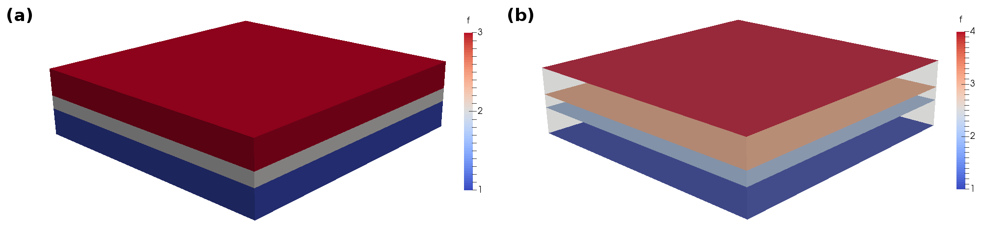
Fig. 20 Domain IDs as displayed by Paraview (a) cell domains (b) facet domains (with threshold filter in order to clip undefined triangles that are displayed as maximum integer value).
Next, we want to assign material parameters to the different domains.
Material parameter assignment in magnum.fe is done by accessing state.material.
Parameters can be set one by one by calling state.material.parameter1 = xxx, state.material.parameter2 = yyy etc. or in bunches by calling state.material = Material(parameter1 = xxx, parameter2 = yyy).
Assigning a value to state.material.parameter will set this value for the complete mesh.
However, more often than not, we want to set different material parameters in different domains.
This can be easily achieved masking (restricting) the material to a certain domain.
# set material parameters in different regions
state.material['top'] = Material(
    alpha = 1.0,
    K_uni = Expression("x[0]*0.5e5")
)
Here, we set two material parameters, namely alpha and K_uni.
While alpha is simply set to the constant value 1 in the ‘top’ region, the material parameter K_uni is given as an spatially varying FEniCS Expression.
Please refer to the FEniCS documentation for details on the use of expressions.
As mentioned easlier, material parameters can also be assigned one by one
state.material['bottom'].K_uni = 1e6
Note, that we do not assign any value for alpha in the ‘top’ region, which leads to a value of 0 in this region.
In order to check the correct parameter assignment we can write the material parameters to PVD files.
# save material paramters to files
File("alpha.pvd") << state.material.alpha
File("K_uni.pvd") << state.material.K_uni
Fig. 21 shows the resulting material parameters in the complete mesh.
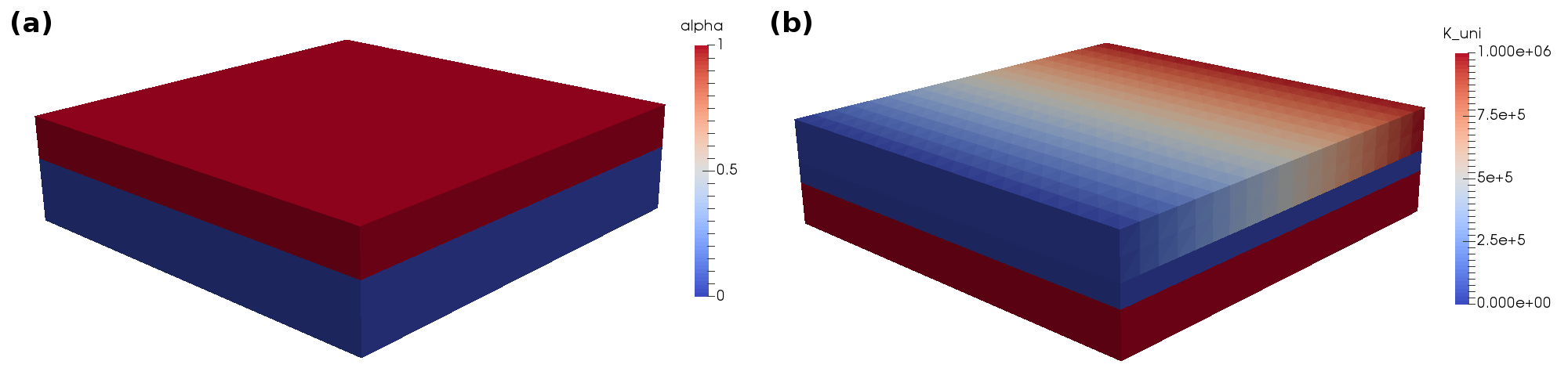
Fig. 21 Material parameters as displayed by Paraview (a) alpha (b) K_uni.
By accessing each domain individually and by the use of Expression objects we already have a very fine grained control over the material parameter assignment.
However, sometimes we might want to go even one step further and directly operate on the mesh level of the material parameters.
Material parameters are discretized with piecewise constant functions which means that there is one material parameter value per mesh cell.
In the following we develop a code that generates a spatially varying anisotropy axis with a uniformly distributed direction.
The code uses the NumPy interface of FEniCS to populate the underlying vectors of the material functions.
An additional challenge is the vector nature of the axis material parameters that requires us to use the split and assign methods to operate on each component individually.
# 1) Initially empty constant
state.material.K_uni_axis = Constant((0,0,0))

# 2) get material function in top domain and split into components
axis_top = state.material['top'].K_uni_axis
axis_top_x, axis_top_y, axis_top_z = axis_top.split(True)

# 3) get number of cells in domain and generate uniformly distributed directions
n_cells = axis_top_x.vector().size()
theta = np.arccos(1. - 2. * np.random.rand(n_cells))
phi   = 2. * np.pi * np.random.rand(n_cells)

# 4) set vectors of components individually
axis_top_x.vector()[:] = np.cos(phi) * np.sin(theta)
axis_top_y.vector()[:] = np.sin(phi) * np.sin(theta)
axis_top_z.vector()[:] = np.cos(theta)

# 5) assign components to vector function and set material
assign(axis_top, [axis_top_x, axis_top_y, axis_top_z])
state.material['top'].K_uni_axis = axis_top

# 6) save result to PVD file
File("K_uni_axis.pvd") << state.material.K_uni_axis
Fig. 22 shows the results for the random distributed anisotropy axes.
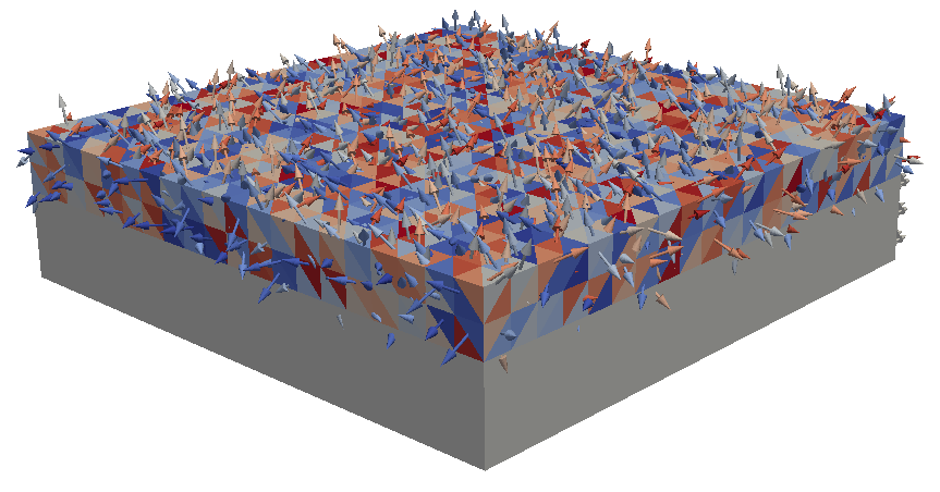
Fig. 22 Random K_uni_axis as displayed by Paraview.
The domain management feature of magnum.fe do not only apply to material parameters but also to state attributes such as the magnetization state.m, the electric current state.j etc.
For example, the State class has a method interpolate that allows to define expresions for the interpolation domain wise.
# set magnetization in different regions
state.m = state.interpolate({
  'bottom': Constant((1.0, 0.0, 0.0)),
  'top': Expression(("cos(x[0])", "sin(x[0])", "0.0"))
})
Here, we choose a constant inplane magnetization in the ‘bottom’ layer and a varying magnetization given by an Expression in the ‘top’ layer.
As for the material parameters, the resulting magnetization can be easily written to a PVD file.
# save magnetization
File("m_complete.pvd") << state.m
File("m_bottom_and_top.pvd") << state.m['bottom_and_top']
While the first command saves the magnetization on the complete mesh into a PVD file, the second command only saves the parts defined by the ‘bottom_and_top’ domain. When dealing with magnetic multilayers that consist of magnetic and nonmagnetic regions this feature can be used to save the magnetization only in physically meaningful (magntic) parts of the structure. The result are depicted in Fig. 23.
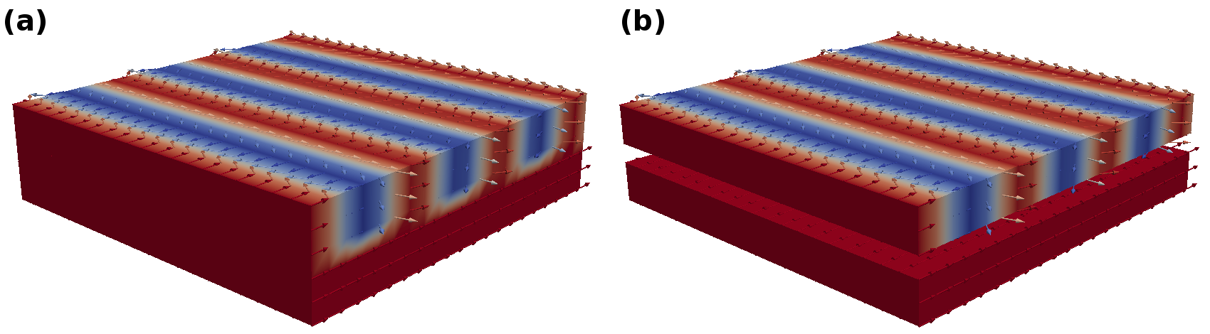
Fig. 23 Magnetization configuration (a) in the complete mesh (b) cropped to a certain region.
As a last example of magnum.fe’s domain management we look at the computation of average values. Both scalar and vector field can be easily averaged over the complete mesh or over certain regions.
# output average magnetization
print state.m.average()
print state.m.average('bottom')
This lead to the following output
(0.520395923452039, 0.014304519185336612, 0.0)
(0.9999999999999999, 0.0, 0.0)
Virtual attributes and field terms
This example shows some useful examples for the handling of Virtual Attributes and Field Terms. We use the same mesh as for the Mesh generation and domain management example.
from magnumfe import *

# create simple, regular box mesh of dimensions 20x20x5
mesh = BoxMesh(Point(0, 0, 0), Point(20, 20, 5), 20, 20, 5)

# create layer regions in z-direction with thicknesses 2,1,2
cell_domain_1 = AutoSubDomain(lambda x: x[2] < 2.001)
cell_domain_2 = AutoSubDomain(lambda x: x[2] > 1.999 and x[2] < 3.001)
cell_domain_3 = AutoSubDomain(lambda x: x[2] > 2.999)
cell_domain_1.mark(mesh, 3, 1)
cell_domain_2.mark(mesh, 3, 2)
cell_domain_3.mark(mesh, 3, 3)

# create facet regions on top/bottom and between the layers
facet_domain_1 = AutoSubDomain(lambda x: near(x[2], 0.0))
facet_domain_2 = AutoSubDomain(lambda x: near(x[2], 2.0))
facet_domain_3 = AutoSubDomain(lambda x: near(x[2], 3.0))
facet_domain_4 = AutoSubDomain(lambda x: near(x[2], 5.0))
facet_domain_1.mark(mesh, 2, 1)
facet_domain_2.mark(mesh, 2, 2)
facet_domain_3.mark(mesh, 2, 3)
facet_domain_4.mark(mesh, 2, 4)

# create state and name domains
state = State(mesh, cell_domains = {
    'bottom': 1,
    'spacer': 2,
    'top': 3,
    'magnetic': (1, 3)
  }, facet_domains = {
    'bottom': 1,
    'spacer1': 2,
    'spacer2': 3,
    'top': 4
  })
Note, that we define a region named “magnetic”, which is the default region name for the magnetic region expected from all field terms and intergrators.
While attributes (and virtual attributes) appear as FEniCS Function object, they are enriched by some convenient methods.
E.g. vector valued attributes, such as the magnetization can be easily normalized with the normalize method.
Averages can be computed with the average method.
# set magnetization and use normalize method to renormalize
state.m = Constant((1.0, 1.0, 0.0))
state.m.normalize()
print "<m> = ", state.m.average()
prints
<m> = (0.7071067811865179, 0.7071067811865179, 0.0)
The magnetization in this case is a regular attribute.
It is a constant vector field that is set by an attribute setter state.m = xxx and can be read afterwards via the attribute getter state.m.
Note, that each Constant, Expression or Function object is interpolated onto a first order discrete Lagrange space (\(\mathcal{P}^1\)) and enriched with methods such as average.
Attributes are used by solvers and field terms to solve the micromagnetic equations.
E.g. the Oersted field term obtains the current for its computations from state.j.
We want to simulate the Oersted field for a current that varies in time.
This is, where virtual attributes come into play.
Virtual attributes can depend on every attribute of the state, including the time, the magnetization or any other normal or virtual attribute.
In the following we define a current that rises from \((0,0,0) \text{A}/\text{m}^2\) at \(t=0\) to \((0,0,10^{12}) \text{A}/\text{m}^2\) at \(t = 1 \text{ns}\).
# define virtual attribute for linearly rising current j
state.j = lambda state: Constant((0, 0, state.t / 1e-9 * 1e12))
state.t = 0.0
print "<j>(0) = ", state.j.average()
state.t = 0.5e-9
print "<j>(0.5e-9) = ", state.j.average()
prints
<j>(0) =  (0.0, 0.0, 0.0)
<j>(0.5e-9) =  (0.0, 0.0, 499999999999.99347)
magnum.fe provides a number of predefined routines to set up virtual attributes.
E.g., the method h() of every field term can be used to directly compute the corresponding field by passing a state object.
# setup simple external field and write to file
external_field = ExternalField(Expression(("x[2]/5./mu0", "0", "0"), mu0 = Constants.mu0))
File("h.pvd") << external_field.h(state)
However, it can also be used a virtual attribute when the state argument is omitted.
# register external field as virtual attribute
state.h_ext = external_field.h()
File("h.pvd") << state.h_ext
One advantage of registering the field method as a virtual attribute, is that virtual attribute, like regular attributes, are enriched with methods such as average.
print "<h_ext> = ", state.h_ext.average()
print "<h_ext>_top = ", state.h_ext.average('top')
print "<h_ext>_top_surface = ", state.h_ext.average('top', 'facet')
prints
<h_ext> =  (397887.35774102324, 0.0, 0.0)
<h_ext>_top =  (636619.7723858159, 0.0, 0.0)
<h_ext>_top_surface =  (795774.7154822319, 0.0, 0.0)
Not only the field method h(), but also the energy method E() of any field term can both be used directly or a virtual attribute.
# compute energy directly and through virtual attribute
state.material.ms = 1.
print "E_ext = ", external_field.E(state)
state.E_ext = external_field.E()
print "E_ext = ", state.E_ext
prints
E_ext =  -565.685424949
E_ext =  -565.685424949
Note, that the material parameter ms has to be set in order to compute the energy.
As another example we register the demagnetization field and check whether the virtual attribute is updated properly on magnetization change.
# create demag field object
demag_field = DemagField()
state.h_demag = demag_field.h()

# check if virtual field attribute is updated on magnetization change
state.m = Constant((1.0, 0.0, 0.0))
print "<h_demag(1,0,0)>_top = ", state.h_demag.average('top')
state.m = Constant((-1.0, 0.0, 0.0))
print "<h_demag(-1,0,0)>_top = ", state.h_demag.average('top')
prints
<h_demag(1,0,0)>_top =  (-0.13839708423953592, -3.3894124376866775e-05, -3.996042348220122e-05)
<h_demag(-1,0,0)>_top =  (0.13839708423953592, 3.3894124376866775e-05, 3.996042348220122e-05)
Another reason to register a field or energy as virtual attribute is its possible use in logger classes.
# use virtual attributes in logger object
logger = ScalarLogger("log.dat", ('t', 'h_ext', 'E_ext', 'h_demag[top]'))
Spin-torque oscillator with restricted integration domain
This example is a variation of the spin-torque oscillator that was introduced in A Simple Spin-Torque Oscillator and requires the same mesh. In contrast to the original version, we want to reduce the computation time by neglecting the dynamics of the fixed layer while still keeping the effects of both the stray field and the spin accumulation onto the free layer. Therefore, we reuse the first part of the original simulation script including the relaxation of the full system.
from magnumfe import *

# read mesh
mesh = Mesh("mesh/stack.xml")

# initialized state
state = State(mesh,
  cell_domains = {
    'electrode_bottom': 1,
    'fixed_layer':      2,
    'spacer':           3,
    'free_layer':       4,
    'electrode_top':    5,
    'magnetic':         (2,4),
    'conducting':       (1,2,3,4,5)
  },
  facet_domains = {
    'contact_bottom':   1,
    'contact_top':      2
  },
  scale = 1e-9
)

# define material constants in magnetic region
state.material['magnetic'] = Material(
  alpha      = 0.1,
  Aex        = 2.8e-11,
  D0         = 1e-3,
  C0         = 1.2e6,
  beta       = 0.9,
  beta_prime = 0.8,
  tau_sf     = 5e-14,
  J          = 4.0e-20
)

# define specific constants for free layer
state.material['free_layer'] = Material(
  ms         = 1.00 / Constants.mu0,
  K_uni      = 0.0,
  K_uni_axis = (0, 0, 1)
)

# define specific constants for fixed layer
state.material['fixed_layer'] = Material(
  ms         = 1.24 / Constants.mu0,
  K_uni      = 1e6,
  K_uni_axis = (0, 0, 1)
)

# define material constants for nonmagnetic region
state.material['!magnetic'] = Material(
  D0         = 5e-3,
  C0         = 6e6,
  tau_sf     = 1e-14,
)

# define start magnetization
state.m = state.interpolate({
            'free_layer':  Constant((1.0, 0.0, 0.0)),
            'fixed_layer': Constant((0.0, 0.0, 1.0))
          })

# initialize field terms
exchange_field = ExchangeField()
demag_field    = DemagField(compute_region = 'all')
aniso_field    = UniaxialAnisotropyField()
external_field = ExternalField(Constant((0.0, 0.0, 0.6 / Constants.mu0)))

# relax the system
llg = LLGCvode([exchange_field, demag_field, aniso_field, external_field])
state.material['magnetic'].alpha = 1.0
for i in range(100): state.step(llg, 1e-11)
Note, that DemagField(compute_region = 'all') is used here instead of DemagField() in the original version.
This means that the complete mesh, including the nonmagnetic domains, is treated with FEM when computing the demagnetization field.
More importantly, the BEM matrix, required for the demagnetization-field computation, is constructed from the outer boundary of the complete mesh, which, in the case of multilayer structures, consists of less nodes than the boundary of the magnetic region.
Since the fixed layer is considered to be static for the rest of the simulation, we can compute its demagnetization field once and reuse this field for the complete simulation.
This can be achieved by creating a DemagField instance with properly set source and target regions and use the computed field in an ExternalField object:
# compute demag_field generated by fixed layer in free layer
# use compute_region = 'all' to avoid BEM matrix reassembly
demag_field_fixed = DemagField(compute_region = 'all',
                               source_region = 'fixed_layer',
                               target_region = 'free_layer')

# create a static field from the fixed-layer demag field
demag_field_fixed_static = ExternalField(demag_field_fixed.h(state))
Since we use compute_region = 'all' again, the BEM matrix does not have to be reassembled but is taken from cache which speeds up the setup and descreases memory requirements.
In a next step we setup a DemagField instance that only solves on the free layer:
# create free-layer only demag field object to save computation time
demag_field_free = DemagField(region = 'free_layer')
Now we setup the spin accumlation solver and hook it into the state as virtual attribute.
# define spin accumulation coupling
spin_acc = SpinAccumulationForCurrent()
state.s  = spin_acc.s()
Note, that we use the SpinAccumulationForCurrent class instead of SpinAccumulationForPotential as in the original script.
Since we do not care about resistance change and the influence of the magnetization configuration onto the electric current is considered to be neglectable, this choice will lead to another performance increase.
The SpinAccumulationForCurrent class expects the current to be provided by state.j
state.j = Constant((0, 0, 4e11))
and as for the original script we need to create a SpinTorque object in order to couple spin accumulation with the magnetization
spin_torque = SpinTorque()
The integrator for the LLG is setup with both the static fixed-layer demagnetization field and the dynamic free-layer field. Furthermore its integration region, which defaults to ‘magnetic’ is set to ‘free_layer` in order to reduce the dimension of the problem.
# create LLG integrator that operates on free layer only
llg = LLGCvode([exchange_field, demag_field_fixed_static, demag_field_free, \
                aniso_field, external_field, spin_torque], region = "free_layer")
The rest of the simulation script is very similar to the original script.
state.material['magnetic'].alpha = 0.1
state.t = 0.0

# prepare log files
logger  = ScalarLogger("log.dat", ('t', 'm[free_layer]'))

while state.t < 5e-9:
  logger  << state
  state.step(llg, 1e-11)
Note, that the electric potential is not logged since it is not computed by the SpinAccumulationForCurrent class.
Fig. 24 shows the simulation results compared to the full simulation from the A Simple Spin-Torque Oscillator section.
The results are slightly different, but important features such as the frequency of the oscillator are very similar to the full fledged simulation.
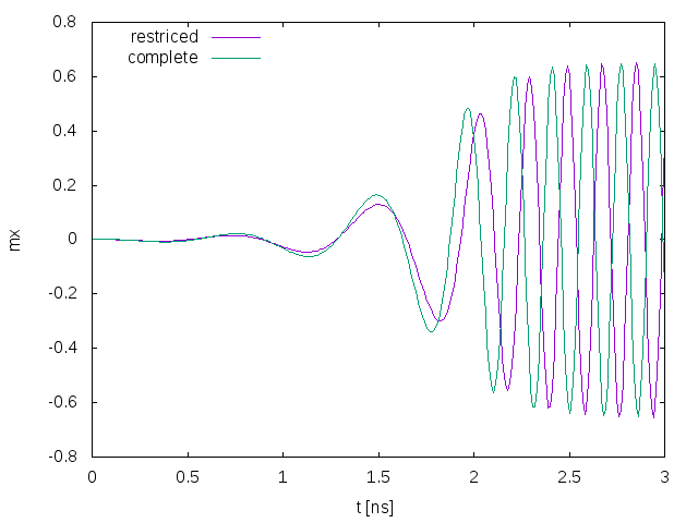
Fig. 24 Oscillator results compared to the full fledged oscillator example.
Spin-torque oscillator with Slonczewski spin torque
This example is a variation of the spin-torque oscillator that was introduced in A Simple Spin-Torque Oscillator. In contrast to the original version, the spin-transfer torque in this example is computed using the model of Slonczewski. The Slonczewski model describes the spin torque in terms of a surface interaction between the neighboring interfaces of the free and fixed layer. In order to set up the solver for the Slonczewski model, the mesh of the original oscillator example has to be modified. The Slonczewski model does not require any leads, however, the neighboring interfaces of the magnetic layers have to be marked with IDs. An appropriate GEO file for Gmsh reads:
cl = 2.5;

Point(1) = {  0,  0, 0, cl};
Point(2) = { 10,  0, 0, cl};
Point(3) = {-30,  0, 0, cl};
Point(4) = { 30,  0, 0, cl};
Point(5) = {  0, 30, 0, cl};
Point(6) = {  0,-30, 0, cl};

Ellipse(1) = {5,1,2,3};
Ellipse(2) = {4,1,2,5};
Ellipse(3) = {6,1,2,3};
Ellipse(4) = {4,1,2,6};

Line Loop(5) = {1,-3,-4,2};
Plane Surface(1) = {5};

s0[] = Extrude{0, 0, 10.0} {Surface{1};     Layers{4};};
s1[] = Extrude{0, 0,  1.5} {Surface{s0[0]}; Layers{1};};
s2[] = Extrude{0, 0,  3.0} {Surface{s1[0]}; Layers{2};};

Physical Volume(1) = {s0[1]};
Physical Volume(2) = {s1[1]};
Physical Volume(3) = {s2[1]};

Physical Surface(1) = {s0[0]};
Physical Surface(2) = {s1[0]};
Fig. 25 shows the resulting domains in the mesh.

Fig. 25 Domain definitions as required by the Slonczewski model (a) Cell domains (b) Facet domains.
The first part of the simulation script is very similar to the original script.
from magnumfe import *

# read mesh
mesh = Mesh("mesh/stack.xml.gz")


# initialized state
state = State(mesh,
  cell_domains = {
    'fixed_layer': 1,
    'spacer':      2,
    'free_layer':  3,
    'magnetic':    (1,3),
  },
  facet_domains = {
    'interface1': 1,
    'interface2': 2
  },
  scale = 1e-9
)


# define material constants in magnetic region
state.material['magnetic'] = Material(
  alpha      = 0.1,
  Aex        = 2.8e-11,
)

# define specific constants for free layer
state.material['free_layer'] = Material(
  ms         = 1.00 / Constants.mu0,
)

# define specific constants for fixed layer
state.material['fixed_layer'] = Material(
  ms         = 1.24 / Constants.mu0,
  K_uni      = 1e6,
  K_uni_axis = (0, 0, 1)
)

# define start magnetization
state.m = state.interpolate({
            'free_layer':  Constant((1.0, 0.0, 0.0)),
            'fixed_layer': Constant((0.0, 0.0, 1.0))
          })
state.j = Constant((0,0,4e11))

# initialize field terms
exchange_field = ExchangeField()
demag_field    = DemagField(compute_region = 'all')
aniso_field    = UniaxialAnisotropyField()
external_field = ExternalField(Constant((0.0, 0.0, 0.6 / Constants.mu0)))

# relax the system
llg = LLGCvode([exchange_field, demag_field, aniso_field, external_field])
state.material['magnetic'].alpha = 1.0
for i in range(100): state.step(llg, 1e-11)
Note, that since we want to use the model of Slonczewski for the spin torque, we don’t require any material parameters connected to the spin-diffusion model (D0, C0, beta, beta_prime, tau_sf, J).
Also the named domains have changed due to the different mesh and a constant current is set in state.j.
Instead of setting up a solver for the spin accumulation, the Slonczewski model is directly implemented as an effective-field term, see SpinTorqueSlonczewski.
# define spin accumulation coupling
spin_torque = SpinTorqueSlonczewski(layer_region = 'spacer',
                                    interface1 = 'interface1',
                                    interface2 = 'interface2',
                                    P = 0.6, Gamma = 0.3)
We use the default bidirectional coupling which requires only the definition of the coupled interfaces and the cell regaion that connects them (spacer).
Furthermore we have to define the constants \(P\) and \(\Gamma\).
The rest of the script is again very similar to the original script.
# solve coupled system
llg = LLGCvode([exchange_field, demag_field, aniso_field, external_field, spin_torque])
state.material['magnetic'].alpha = 0.1
state.t = 0.0

# prepare log files
logger  = ScalarLogger("log.dat", ('t', 'm[free_layer]'))
mlogger = FieldLogger("data/m.pvd", 'm[magnetic]', every = 10)

while state.t < 15e-9:
  logger  << state
  mlogger << state
  state.step(llg, 1e-11)
Fig. 26 shows the simulation results as computed by magnum.fe.
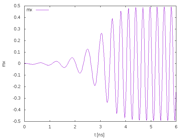
Fig. 26 Oscillator results obtained with the Slonczewski model.
Energy barrier computation of magnetic multilayer with the string method
In this example the energy barrier between the parallel and antiparallel state of an elliptical multilayer structure is computed.
First we use Gmsh to create an appropriate mesh.
The geo file stack.geo for a trilayer with thicknesses 10nm, 1.5nm, 3nm and radii 40nm and 15nm respectively reads:
cl = 3.0;

Point(1) = {  0,  0, 0, cl};
Point(2) = { 10,  0, 0, cl};
Point(3) = {-40,  0, 0, cl};
Point(4) = { 40,  0, 0, cl};
Point(5) = {  0, 15, 0, cl};
Point(6) = {  0,-15, 0, cl};

Ellipse(1) = {5,1,2,3};
Ellipse(2) = {4,1,2,5};
Ellipse(3) = {6,1,2,3};
Ellipse(4) = {4,1,2,6};

Line Loop(5) = {1,-3,-4,2};
Plane Surface(1) = {5};

s0[] = Extrude{0, 0, 10.0} {Surface{1};     };
s1[] = Extrude{0, 0,  1.5} {Surface{s0[0]}; };
s2[] = Extrude{0, 0,  3.0} {Surface{s1[0]}; };

Physical Volume(1) = {s0[1]};
Physical Volume(2) = {s1[1]};
Physical Volume(3) = {s2[1]};
A magnum.fe compatible mesh file is generated by calling Gmsh and converting the resulting mesh:
gmsh -3 stack.geo
magnum.msh stack.msh stack.xml.gz
Note that we use the file extension xml.gz here leads to compressed output.
The simulation script for the energy-barrier computation starts as any magnum.fe simulation script by importing the magnumfe library:
from magnumfe import *
Next we import the mesh and create a State object with named domains:
# create mesh and state
mesh  = Mesh("stack.xml.gz")
state = State(mesh, cell_domains = {
    'magnetic': (1,3),
    'fixed': 1,
    'free': 3
  }, scale = 1e-9)
Only the upper and lower layers are defined as magnetic. The middle layer is not named since it is not required for the energy computation. The material parameters \(M_\text{s}\) and \(A\) are assigned to the magnetic regions in order to compute the energy due to the demagnetization and exchange field.
state.material['magnetic'] = Material(
    ms  = 8e5,
    Aex = 1.3e-11
  )
Note, that it is not required to assign \(\alpha\) since we are not interested in the dynamics of the system but only in the energy barrier.
Now, we initialize the StringSolver object, by defining the desired energy contributions and the state for the computations.
string = StringSolver(state, [
    ExchangeField(),
    DemagField()
  ])
The string solver iteratively relaxes a magnetization trajectory between two minima in order to find the minimum energy barrier.
This trajectory is discretized by a number of magnetization images.
This number can be configured when initialized the StringSolver object and defaults to 20.
In order to create a start trajectory with \(N\) (in this case 20) images you can call the level method on an arbitrarily sized list of magnetization images.
We want to start from an out-of-plane rotation from parallel to antiparallel which can be easily parametrized by three images (1: parallel, 2: out-of-plane, 3: antiparallel)
images = string.level([
  state.interpolate({'fixed': Constant((1,0,0)), 'free': Constant(( 1,0,0))}),
  state.interpolate({'fixed': Constant((1,0,0)), 'free': Constant(( 0,0,1))}),
  state.interpolate({'fixed': Constant((1,0,0)), 'free': Constant((-1,0,0))})
])
This initial trajectory leads to a very high energy barrier since the out-of-plane configuration is highliy unfavorable due to the shape anisotropy.
The string method is expected to optimize this trajectory to an in-plane rotation with possibly non-homogeneous magnetization configurations.
The StringSolver object operates on the images object and changes it iteratively.
In order to log the optimization process we generate two log files barrier.dat and energies.dat.
In barrier.dat we save the energy barrier measured from both energy minima (parallel and antiparallel state).
In energies.dat we save the energies of the complete trajectory for every string-method iteration.
bfile =  open("barrier.dat", "w", 0)
efile =  open("energies.dat", "w", 0)
Furthermore, we create some variables/constants to monitor the minimization process
i = 0           # step counter
etol = 1e-23    # stop criterion (energy barrier change in Joule)
delta_e = 1e99  # start value for energy barrier
Now we enter the optimization loop.
Within the loop, the step method is called on the StringSolver object, performing one optimization iteration on the images object.
After each simulation step the results, including all magnetization iamges, are written in different log files.
Furthermore the energy barrier is computed and compared to the last iteration.
If the change in the energy barrier is less than etol, the optimization is considered to be converged.
# loop until convergence
while abs(max(images.E) - min(images.E) - delta_e) > etol:

  # update value of energy barrier for stopping criterion
  delta_e = max(images.E) - min(images.E)

  # perform string method step (relax every image for 2e-11 s)
  string.step(images, 2e-11)

  # write all magnetization images
  mfile = File("step_%d/m.pvd" % i)
  for m in images: mfile << m['magnetic']

  # write all energies (step no, image no, energy)
  for j, e in enumerate(images.E): efile.write("%d %d %g\n" % (i, j, e))
  efile.write("\n")

  # write energy barriers (step no, first image to max, last image to max)
  bfile.write("%d %g %g\n" % (i, max(images.E) - images.E[0], max(images.E) - images.E[-1]))

  # increase step counter
  i = i + 1
Finally, we close the log files by calling
bfile.close()
efile.close()
The results logged in energies.dat and barrier.dat are shown in Fig. 27 and Fig. 28 respectively.
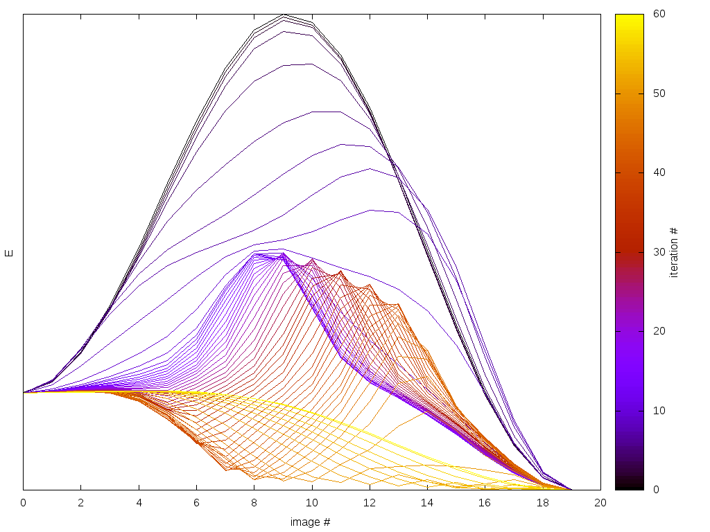
Fig. 27 Transition-path energies for different string-method iterations.
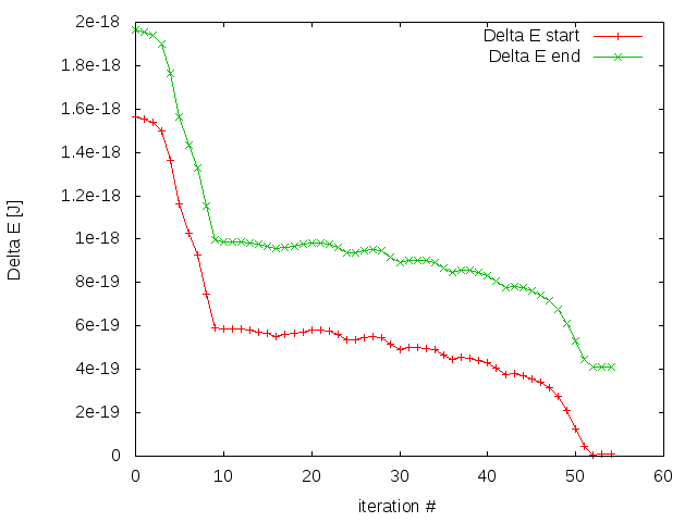
Fig. 28 Energy barrier evolution during string-method iteration.