Getting Started

As a first example the standard problem #4 [MuMag4], proposed by the MuMag group is computed with magnum.fe. This problem describes the switching of a thin strip of permalloy under the influence of an external field.

The Standard Problem #4

Since magnum.fe is a Python library, a simulation script is a Python script that imports magnum.fe. Thus, every magnum.fe simulation script starts with

from magnumfe import *

In the next step a mesh for the simulation is created. For simple geometries, the meshing tools of FEniCS are a good choice. More complicated geometries can be meshed with external tools. magnum.fe comes with the mesh converter magnum.msh that supports a variety of file formats through the Gmsh library. Depending on the method for the solution of the open-boundary demagnetization field problem, the mesh is also required to include a cuboid shell, see Open Boundary Problems.

Here we use the hybrid FEM-BEM method, see Hybrid FEM-BEM Method (Fredkin and Koehler), for the computation of the demagnetization field. Hence a simple cuboid mesh as provided by the FEniCS meshing tools is sufficient for the solution of the standard problem #4, that requires a cuboid of size \(500 \times 125 \times 3\) nm. The mesh is constructed symmetrically around the coordinate origin and scaled by \(10^9\).

mesh = BoxMesh(Point(-250, -62.5, -1.5), Point(250, 62.5, 1.5), 100, 25, 1)

A magnetization configuration that is known to relax quickly in a magnetic s-state is defined by an analytical expression. Note, that magnum.fe expects the magnetization to be normalized to 1.

m0 = Expression(("cos(a)", "sin(a)", "0.0"), a=Expression("fabs(pi*x[0]/1e3)"))

A simulation state is created and initialized with material parameters and the start magnetization m0. Note that the scale parameter is set to \(10^{-9}\) since the problem size is given in nanometers. This scaling is advised to avoid numerical artifacts.

state = State(mesh, material = Material.py(), scale = 1e-9, m = m0)

For the relaxation of the system, an LLG-solver object is created that includes the exchange field and demagnetization field as only effective field contributions. From the available integration routines the fully implicit LLGCvode solver is by far the fastest.

exchange_field = ExchangeField()
demag_field    = DemagField()
llg = LLGCvode([exchange_field, demag_field])

The system is relaxed by setting the damping of the material to \(\alpha = 1\) and performing a number of integration steps.

state.material.alpha = 1.0
for i in range(100): state.step(llg, 1e-11)

In order to switch the magnetization as required by the standard problem #4, the damping is reduced to \(\alpha = 0.02\). A new solver object is created that reuses the exchange field demagnetization field objects and additionally includes an external field. Furthermore the simulation time is reset to 0.

state.material.alpha = 0.02
state.t = 0.0
external_field = ExternalField(Constant((-24.6e-3/Constants.mu0, +4.3e-3/Constants.mu0, 0.0)))
llg = LLGCvode([exchange_field, demag_field, external_field])

Note that magnum.fe expects all field values to be given in A/m. To convert from Tesla just divide by Constants.mu0. The time loop for the solution of the LLG is programmed as Python while loop. Before entering the integration loop we define some log files. Here we use two log files. In the first file log.dat we want to write the averaged magnetization for every time step. The logging of scalar values in magnum.fe can be realized with the ScalarLogger class. The second file should contain the complete magnetization configuration for different times, which can be implemented with the FieldLogger class. Since this leads to the creation of large amounts of data we want this logger to log only every 10th step.

# prepare log files
logger  = ScalarLogger("log.dat", ('t', 'm'))
mlogger = FieldLogger("data/m.pvd", 'm', every = 10)

The loop for integration of 1 ns with logging then reads

# loop, loop, loop
while state.t < 1e-9:
  logger  << state
  mlogger << state
  state.step(llg, 1e-12)

Complete code

from magnumfe import *

# generate mesh
mesh = BoxMesh(Point(-250, -62.5, -1.5), Point(250, 62.5, 1.5), 100, 25, 1)

# define start magnetization
m0 = Expression(("cos(a)", "sin(a)", "0.0"), a=Expression("fabs(pi*x[0]/1e3)"))

# initialize state
state = State(mesh, material = Material.py(), scale = 1e-9, m = m0)

# create exchange and demag field objects
exchange_field = ExchangeField()
demag_field    = DemagField()

# initialize llg integrator and relax the system to s-state with high alpha
llg = LLGCvode([exchange_field, demag_field])
state.material.alpha = 1.0
for i in range(100): llg.step(state, 1e-11)

# reset alpha and initialize LLG integrator with external field
state.material.alpha = 0.02
external_field = ExternalField(Constant((-24.6e-3/Constants.mu0, +4.3e-3/Constants.mu0, 0.0)))
llg = LLGCvode([exchange_field, demag_field, external_field])

# prepare log files
logger  = ScalarLogger("log.dat", ('t', 'm'))
mlogger = FieldLogger("data/m.pvd", 'm', every = 10)

# loop, loop, loop
while state.t < 1e-9:
  logger  << state
  mlogger << state
  state.step(llg, 1e-12)

Run the Simulation

Since the simulation file is a simple Python script it is run with the Python interpreter. Save the above program to a file called sp4.py and run

python sp4.py

on the command line.

Watch the Results

This simulation produces a textfile with whitespace separated values of the time and the averaged magnetization components in it named log.dat. A simple way to visualize these results is the plotting tool Gnuplot which is installed in magnum.fe virtual machine image. In the simulation directory open Gnuplot by typing

gnuplot

This opens a gnuplot console. The results from the log.dat file can be plotted by typing the following commands.

set xlabel "t [s]"
set ylabel "m"
plot "log.dat" using 1:2 with lines title "mx", \
     "log.dat" using 1:3 with lines title "my", \
     "log.dat" using 1:4 with lines title "mz"

This should bring up a window with the averaged magnetization components plottet over time, see Fig. 4. For more information on Gnuplot, please refer to the online manual at http://www.gnuplot.info/.

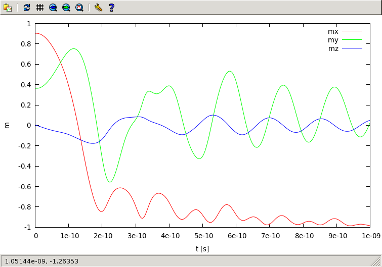
Fig. 4 Results for the standard problem #4 plotted with Gnuplot

Additionally, the full magnetization configuration is written to a PVD file every 10th time step. This file can be opened with any VTK viewer, e.g. Paraview.

The Next Steps

The following sections of the manual will walk you through more advanced topics such as mesh generation and problem definition on multi-domain structures. These tutorial like sections will be followed by reference sections that give you an overview over all existing classes and functions.

Since magnum.fe is based on the finite-element library FEniCS, all functionality of FEniCS is also available in magnum.fe simulation scripts. In particular all spatially varying fields such as the magnetization are FEniCS Function objects and can be processed by FEniCS routines. Please refer to the FEniCS documentation under http://fenicsproject.org/documentation/ in order to make use of this functionality.

If you installed the virtual machine image of magnum.fe, you will find an examples directory that contains a number of useful demo simulation scripts, including the examples described in this manual.

[MuMag4]

µMAG Standard Problem #4, http://www.ctcms.nist.gov/~rdm/std4/spec4.html